How to Optimize AWS S3 Costs via Granular Visualization

What happens when a data lake turns into a data swamp. Credit: Photo by Krystian Piątek on Unsplash

TL;DR: Expressive visualisations help to save money. For example, if you’re using S3 as your cloud storage of choice, then S3 Server access logs show who accessed which S3 object. S3 Inventory regularly exports the metadata of each S3 object in your bucket. These two data sources can be used to answer questions like “How much does this prefix cost per month?”, “How frequently was this prefix accessed for past 30 days?”, or “How much will it cost to transfer this prefix to Glacier?” Go collect and join this data. Then, build treemap visualizations for insights on your spending.

Wow, that’s a huge cloud bill!

Companies build remarkable AI products that store and process a lot of data. Data is the new oil, they say. But how do we make sure we don’t spend too much on oil tanks?

Many data-driven companies have been there. To provide intelligent products, they need to be trained on significant volumes of data. So, they build a data lake. They save every single useful event, message, log, etc., hoping to extract value from it later on. Data engineers build sophisticated pipelines. There are tables that depend on other tables (some get deprecated, and others are unused). Basically, it all eats up a lot of space.

This is one of many ways a data lake can become a data swamp, which is hard to manage and usually costs a lot of money to maintain.

In this article, we’ll explore techniques that can help cloud infrastructure owners figure out how to clean up data. We’ll explore ways of solving problems in AWS and similar techniques that can be replicated in other cloud providers with similar APIs. I’ll add some links to the APIs that can be used if you use Azure or GCP.

Source of inspiration

As a macOS user and a software engineer, I sometimes struggle with my hard drive running out of space. There’s another similar problem: here’s a folder that consumes a lot of space. Why is it so heavy? What consumes that precious disk space?

To solve this problem locally, I use a tool called DaisyDisk. (There are probably many similar tools, even for other operating systems — e.g., WinDirStat of Windows.)

What is so cool about this tool is the visualization technique it uses to represent disk space. It’s called a sunburst graph. Here are some examples of how it can be built using Plotly:

Definition of Done

Building the sunburst visualization for S3 buckets would help us find the most expensive S3 folders to examine their cost and data size.

But we can do even better than that. What if we could see who accessed files from any given S3 prefix, including how frequently? We can build that visualization as well.

It’s also important to note that costs come not only from storage. We also pay for API requests to the storage infrastructure. If a big chunk of the AWS S3 bill comes from API requests, then how can we figure out what causes it? We can build the prefix to request visualization.

In this article, we’ll build:

• A sunburst graph of the S3 bucket that visualizes the money we spend on each prefix
• A visualization of the usage of each S3 prefix
• A visualization of the frequency of requests to each S3 prefix

Data sources

We will use Python + PySpark for data processing and boto3 Python library for accessing the AWS API, but the logic can be replicated in any programming language. Make sure that the data processing framework you use can fit significant amount of logs. (For example, Pandas will choke when analyzing buckets with too many objects.)

To accomplish this task, we need to answer two types of questions for each S3 object:

• How much does it cost to store this object per month?
• How many requests have been done to this object for the past X# days?

S3 Server access logs and the S3 Inventory will help us answer these questions.

Other cloud providers have similar capabilities, but the APIs and data sources might be different. For example, Azure has blob inventory and storage analytics logging. GCP has storage inventory reports and access logs.

Step 0: Learn about the costs in your AWS region

First, we need to learn how much S3 charges us for requests/storage in our region. These costs differ from region to region. Learn yours on the AWS website.

Note that the costs are per storage class. Each storage class provides different sets of tradeoffs.

Another option is to use the API to fetch up-to-date prices.

from mypy_boto3_pricing import PricingClient

pricing: PricingClient = boto3.client('pricing')
pricing.get_products(
    ServiceCode='AmazonS3',
    Filters=[ 
      { 
         "Field": "regionCode",
         "Type": "TERM_MATCH",
         "Value": "us-east-1" # Change to your favourite region.
      }
    ]
)

The S3 pricing is sophisticated, but in this article, we’re interested in two cost components. Depending on the S3 Storage class of the object, we pay different rates for:

• Storage (pay for GB per month)
• Requests [pay for 1000 requests, GETs, COPYs, Lifecycle transitions and data retrieval requests (change of storage classes)]

For a given object, we know:

• its size
• its storage class
• how many requests of each type were done to it for a past month

From that, we know how much this object costs us per month (the prices from step 0) and if it makes sense to delete or move it to another storage class.

Step 1: Learn about the storage (and storage costs)

The AWS API already supports retrieving all the metadata about specific S3 objects:

import boto3
from mypy_boto3_s3 import S3Client

s3: S3Client = boto3.client('s3')
resp = s3.head_object(
    Bucket='my-bucket',
    Key='some/file.txt'
)
print(resp['StorageClass'], resp['ContentLength'])

This works if you need to fetch this metadata for thousands of objects. But what if your bucket has millions of objects, and you want this metadata to be updated daily? On a daily basis, this would cost us:

object_count / 1000 * cost_of_1000_head_requests

And it will also work painfully slow because of the amount of daily requests we might have to make to fetch all metadata.

Luckily, S3 already provides us with a great tool to dump all of this metadata daily. It’s called S3 Inventory.

Parquet is the preferred data format.

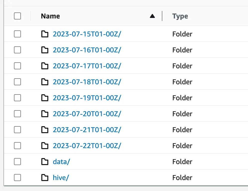
You can create per-bucket Inventory configuration in the Management section of S3 bucket. When enabled, S3 generates a report with the following file structure. Each timestamp prefix contains a manifest with a list of files from data/ folders that represent the state of the bucket for a given timestamp. data/contains files. (Note: This is in the format that you picked during configuration. I picked Apache Parquet.)

This is the prefix that is updated by the S3 Inventory.

To read this report, you can use AWS Athena or manually parse the manifest for a given data and read corresponding files. I use Apache Spark to read and process the files (and assume that SparkSession spark exists) because their size can be significant.

from mypy_boto3_s3 import S3ServiceResource
import json

s3 = boto3.resource('s3')

object = s3.Object(
    'some-bucket',
    '.../2023-07-22T01-00Z/manifest.json').get()['Body'].read()
manifest = json.loads(object)

bucket = manifest['destinationBucket'][len('arn:aws:s3:::') :]
file_keys = [f['key'] for f in manifest['files']]
files = [f's3://{bucket}/{key}' for key in file_keys]

# We use Apache Spark to read manifest files. You can use
# any other approach that is suitable for you.
s3_inventory = spark.read.parquet(*files)
# Here we preprocess this data and store the result as parquet dataframe.
(
    s3_inventory.withColumn('parts', F.split(F.col('key'), '/'))
    .withColumn('full_path_length', F.size(F.col('parts')))
    .select(
        F.explode(F.sequence(F.lit(0), F.size(F.col('parts')))).alias('path_length'),
        F.array_join(F.slice(F.col('parts'), F.lit(1), F.col('path_length')), '/').alias(
            'prefix'
        ),
        (F.col('path_length') == F.col('full_path_length')).alias('is_file'),
        F.col('bucket'),
        F.col('storage_class'),
        F.col('intelligent_tiering_access_tier'),
        F.col('size'),
    )
    .write
    .parquet(...)
)

We have a daily updated dataset that contains metadata for all S3 objects in the given bucket. Note that for an object with key a/b/c.txt, the resulting DataFrame will have 4 rows with path_length equal to 0, 1, 2, and 3 along with corresponding prefixes a, a/b, and a/b/c.txt. This is required to group this data frame by prefix and aggregate total sizes and storage costs.

Moreover, the logs contain the following important fields:

• bucket and prefix — the object that is being manifested
• storage_class — the S3 Object storage class
• intelligent_tiering_access_tier — if storage_class is Intelligent-Tiering, this field defines the tier
• size — the file size

Step 2: Collect object access data

The S3 bucket Properties section provides S3 Server access logs settings, where you can configure exporting S3 object access events. They are exported as CSV files with about 1 minute latency.

S3 Server access logging settings.

The format of the logs is described here. Here’s how to read the logs using Apache Spark:

RAW_CSV_SCHEMA = schema = StructType([StructField(f'_c{idx}', StringType()) for idx in range(25)])

def read_bucket_logs(spark: SparkSession, bucket: str, path: str, day: date):
    return (
        spark.read.option('header', False)
        .option('delimiter', ' ')
        .schema(RAW_CSV_SCHEMA)
        .csv(os.path.join(path, f'{day.isoformat()}-*'))
        .select(
            f.col('_c0').alias('owner').cast(StringType()),
            f.col('_c1').alias('bucket').cast(StringType()),
            f.to_timestamp(
                f.substring(f.concat(f.col('_c2'), f.lit(' '), f.col('_c3')), 2, 26),
                'dd/MMM/yyyy:HH:mm:ss Z',
            ).alias('time'),
            f.col('_c4').alias('ip').cast(StringType()),
            f.col('_c5').alias('requester').cast(StringType()),
            f.col('_c6').alias('request_id').cast(StringType()),
            f.col('_c7').alias('operation').cast(StringType()),
            f.col('_c8').alias('key').cast(StringType()),
            f.col('_c9').alias('request_uri').cast(StringType()),
            f.col('_c10').alias('http_status').cast(IntegerType()),
            f.col('_c11').alias('error_code').cast(StringType()),
            f.col('_c12').alias('bytes_sent').cast(LongType()),
            f.col('_c13').alias('object_size').cast(LongType()),
            f.col('_c14').alias('total_time_millis').cast(LongType()),
            f.col('_c15').alias('turnaround_time_millis').cast(LongType()),
            f.col('_c16').alias('referer').cast(StringType()),
            f.col('_c17').alias('user_agent').cast(StringType()),
            f.col('_c18').alias('version_id').cast(StringType()),
            f.col('_c19').alias('host_id').cast(StringType()),
            f.col('_c20').alias('signature_version').cast(StringType()),
            f.col('_c21').alias('cipher_suite').cast(StringType()),
            f.col('_c22').alias('authentication_type').cast(StringType()),
            f.col('_c23').alias('host_header').cast(StringType()),
            f.col('_c24').alias('tls_version').cast(StringType()),
        )
        .withColumn('day', f.lit(day))
        .withColumn('bucket', f.lit(bucket))
    )

With this data frame, we can do the same trick as with inventory, where we aggregated the dataset by path and path_length. Note that the logs contain the following important fields:

• bucket and prefix — the object that is being manifested
• time — the timestamp when the request occurred
• requester — the IAM role of the subject, who made the request
• operation — the S3 operation

Step 3: Join and visualise

We ended up with two datasets:

• Inventory dataset: keyed by bucket and prefix. Contains aggregate storage sizes per each storage class. Costs for storage per month storage_cost_per_month. (Remember Step 0? Multiply the storage sizes by the cost per storage class, and you’ll get the storage cost.)
• Server access logs dataset: keyed by bucket and prefix. Contains an aggregate number of Tier 1 and Tier 2 requests per path. requests_cost_per_month costs for requests to prefix per month. (Multiply the number of requests by the cost per 1000 requests from Step 0.) log_access_count_30d is the logarithm of the number of requests for the given prefix.

When we join the datasets by bucket and prefix, we’ll have all the data to visualize the bucket costs. Furthermore, we add a column parent_prefix , which is equal to the folder, that contains the folder/object in prefix (e.g., for prefix=a/b/c parent_prefix=a/b).

Let’s use the plotly library to visualize the storage costs. The following call creates the visualization. Note that you can filter the df with a particular prefix and limit the depth (the number of inner folders) of visualization, as the rendering can be taxing for the web browser.

import plotly.express as px

px.treemap(df, 
    names='prefix',
    parents='parent_prefix',
    values='storage_cost_per_month',
    color_continuous_scale='RdBu',
    color='log_access_count_30d',
    branchvalues='total')

The same trick can be done with requests (just replace storage_cost_per_month with requests_cost_per_month):

Did you notice the grey rectangles in the storage costs visualization? Grey comes from the color argument of the px.treemap call and means that the prefix hasn’t been accessed for the past month. These prefixes are great candidates for removal or another storage class transition.

Conclusion

The proposed way of visualization of S3 bucket costs can save a significant amount of funds by making S3 observability more granular. I managed to save dozens of thousands of dollars on cloud bills using these data sources, and at Constructor, we managed to save up to 40% of S3 costs using this technique. I suggest you try it as well.