Training Convolutional Neural Networks to assist pathologists
My approach to the Tumor Proliferation Assessment Challenge
Motivation
I have been meaning to get some hands-on experience with deep learning frameworks for a while now, and I love working on challenging problems in healthcare. So when I heard about TUPAC last summer, I decided to give it a try. TUPAC stands for Tumor Proliferation Assessment Challenge (if you are here because of your love of rap music, I’m afraid you will be disappointed).
It is a computer vision challenge in which the goal is to train algorithms that could be useful for breast cancer prognosis. Some of the code I wrote for this challenge is available here. My Dockerfile is available here. This post requires a basic understanding of deep learning for computer vision, a great resource to study up on this is Stanford’s CS231n.
The Problem
When a patient is diagnosed with breast cancer, an accurate prognosis is needed to inform what treatment should be chosen (the more aggressive the tumor, the more aggressive the treatment). This prognosis is performed by clinical pathologists, by examining histological slides that were obtained through a biopsy. Under the microscope, they look for the density of mitoses in the cancer tissue, since mitoses are a good biomarker for how fast the tumor will spread. However, this mitosis counting method suffers from high subjectivity which leads to low reproducibility. This is a problem that might be remedied by using more objective automated methods. If you want to learn more, the challenge website is a good place to start.
The Dataset
The TUPAC organizers provided a 490 GB dataset consisting of 500 breast cancer cases (taken from The Cancer Genome Atlas). The dimensions of the images can exceed 50,000 by 50,000 pixels. The images are stored in the .svs Aperio file format, which is a special format developed for pyramidal multi-resolution access to pathology images. Each case is labeled with 2 proliferation scores: one based on mitosis counting by pathologists and one based on the RNA expression of 11 genes associated to proliferation. Let’s call the former the human score and the latter the molecular score. The human score is an ordinal number ranging from 1 (good prognosis) to 3 (bad prognosis).
The organizers also made a couple of auxiliary datasets available, one to train a model for mitosis counting and one to train a model for region of interest (ROI) detection. The thought behind this is to train a composite model that performs these subtasks (ROI detection and mitosis counting in the ROIs) to arrive at the proliferation score. Because of time constraints I decided to try to train a model on the main dataset that would directly predict the proliferation scores.
Identifying Regions of Interest
Since the images have very high dimensions, it would not be feasible to feed them to a neural network in their original resolution. But we need to maintain enough detail in order to be able to discern the individual mitoses. So it’s a good idea to first zoom in on certain ROIs, i.e. zones that have a high prognostic value (usually because of high mitotic activity). As mentioned earlier, the organizers provided a separate dataset with annotated ROIs, to train a model to automatically locate ROIs. Instead of training a separate model, I took a different approach inspired by a recent Nature paper by Yu et al. The authors of this paper identified ROIs based on image density.
First I transformed the image into a binary image where pixels that have all RGB values under 200 are 0 and the other pixels are 1. Then I tiled the image into patches of 1024 pixels that overlapped by 512 pixels. For each patch, the density is calculated as the percentage of pixels that are 1. Patches close to the border are ignored because there is often a shadow present. To ensure that the patches aren’t too close to each other, I enforced that the Manhattan distance between all ROIs would be at least 4 times the patch size. Finally, I select the 10 densest patches in the images to be my ROIs.
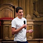
The image below shows the ROIs that were selected by this approach in green, and the ROIs that were annotated by the human pathologists in yellow. At first sight they seem to be located far away from each other. This is not always the case though, in a lot of the slides the human ROIs and the ROIs selected by the algorithm are very close to each other.
When we inspect the ROIs more closely (see image below), we can see that the ROI that is selected by the algorithm is noticeably ‘darker’ than the random region. This could mean that there is a lot of mitotic activity going on there, or it could be caused by the presence of tumor-infiltrating lymphocytes (which have also been shown to have prognostic value).
Training Neural Networks
Now that I have reduced the whole slide images to a couple of smaller ROIs, it’s time to start playing with some CNNs. I used the Keras library with a TensorFlow backend, because it’s very easy to get started with and it seems to be one of the more popular libraries for deep learning competitions.
Since there are multiple ROIs per slide (I started out with 10 but moved it down to 5 to speed up computation), I decided to try out an architecture that can take all these ROIs as input simultaneously. Inspired by this blogpost by Jeffrey De Fauw, I decided to combine the dense representations of the ROIs as inputs to a fully connected softmax layer. Because the human proliferation score is a discrete number, I had to map the continuous outputs from the regression to discrete scores. To do this, I used the decoding method described here by Chenglong Chen.

The architecture I started out with for the individual ROIs was adapted from the ResNet50 implementation for Keras. The Residual Learning framework was introduced in 2015 by He et al. I had seen a couple of papers that applied it successfully, so I was hopeful that it would perform well here too. Next, I got busy optimizing my ResNet implementation to run on multiple GPUs. I added feature-wise standardization and normalization, and started thinking about data augmentation, implementing a custom loss function, class balancing and optimizing other hyperparameters. It was a classic case of premature optimization.
When I started training my architecture on the training dataset, it turned out that my learning curves were not going down at all. They started out at a pretty low mean squared error after one epoch, but never improved upon that initial error. The advice I got from Daniel Hauagge, who was a Runway Postdoc at Cornell Tech at the time, was to start with a very simple architecture and then gradually improve upon that. So I started with something along the lines of AlexNet, but played around with the amount of convolutional layers to see what would perform best. I got the best results for 3 convolutional layers, and when I added too many layers the learning curves would flatline again. My AlexNet-inspired architecture that used 3 convolutional layers for each ROI and then merged the dense representations was learning, but the evaluation metrics were far from impressive.
Because it would be more efficient to predict the human and the molecular proliferation score simultaneously, I started out with one model that had 2 outputs. Decoupling the model into a separate one for each proliferation score had a positive impact, which hints that there is not a lot of agreement between the two scores. To be fair, if there was, there wouldn’t really be a need for automated methods. The organizers also used 2 different evaluation metrics — quadratic weighted Cohen’s kappa for the human score and Spearman’s correlation coefficient for the molecular score — which was another argument in favour of decoupling. At this point, the performance for predicting the molecular proliferation score was getting closer to what would be relevant in a clinical setting (although still not great), while the performance for the human score was still very disappointing. For this reason, I decided to focus on just predicting the molecular proliferation score for now.
The table below shows the architecture I ended up using (shown here for 3 ROIs instead of 5, to save space). There is a branch for each ROI consisting of 3 sequences of convolutional layers. After each convolutional layer, a ReLU activation function is applied, as well as batch normalization. Max pooling is applied after the first and third convolutional layers. These branches end with a fully-connected layer. Eventually the branches are merged, and the result is fed into a final fully-connected layer.
One possible reason for the high mean squared error could have been the ROI selection algorithm. To test this hypothesis, I trained my model on the cases for which the organizers provided ROIs that were selected by pathologists. This reduced the (already small) dataset from 500 to 148 cases. In order to counter this, I should have probably used more elaborate data augmentation (rotations, but als translations around the ROI centroid) and class balancing. Since the organizers provided around 3 ROIs per case, I switched my model to be trained on 3 inputs. When trained on the 148 cases with given ROIs, the model achieved similar performance as when I trained it on the 500 cases with the automatically selected ROIs. This makes me believe that I could have further improved my model’s performance by applying more data augmentation on the 148 cases with given ROIs, or by improving my ROI selection algorithm. Sadly, I had run out of time by this point, so I had to settle for a Spearman’s correlation coefficient of 0.29 (the results of the 5 submitting teams ranged from 0.474 to 0.617).
What should I have done differently?
Lunit Inc. have achieved the best results for both tasks in this challenge (and the additional mitosis counting task that was added later on). I’m very much looking forward to the writeup of their methods, and will update this blogpost with a link when they post it. In the meantime, here are some ideas I have about possible improvements. If any of you want to post feedback/tips for me in the comments, that would be very much appreciated!
First of all, I should have made better use of the limited dataset. I already mentioned data augmentation above. Another approach could have been to not merge all the ROIs for one case, but to train a model on single ROIs and then merge the predictions for the ROIs with some sort of voting mechanism. This would decrease the amount of parameters in the model, and since there are a large amount of ROIs that could be taken out of each slide it would drastically increase the amount of instances the model is trained on. With more data, it is also plausible to assume that more elaborate architectures would show better results.
The second possible improvement would be to train a composite model, that explicitly goes through the steps that a pathologist undertakes: first identify a ROI, then count the mitoses in that ROI, finally combine the information in all ROIs. There are a number of people that have already shown good results for mitosis counting with Convolutional Neural Networks (CNN’s), e.g. Wang et al. The team from The Harker School seems to have applied a strategy similar to this, their writeup is available here.
It would probably also have been smarter to use transfer learning instead of training the network from scratch. This repo makes CNN’s available that are pre-trained on the ImageNet Dataset, implemented in Keras. This would have sped up the learning process and probably would have resulted in better performance. Since this pathology dataset is rather different from ImageNet, the correct approach would probably have been to fix the weights in the first layers and finetune the other layers on the pathology dataset.
Finally, the Expectation-Maximization approach that is described here by Hou et al. would have also been worth a try.
Thanks
I’ve had a lot of fun working on this challenge, and definitely learned a lot. In the future, I will be looking for other interesting deep learning challenges, especially in pathology, radiology and ophthalmology.
I’m grateful to the researchers from Eindhoven University of Technology, University Medical Center Utrecht, Beth Israel Deaconess Medical Center and Harvard Medical School for organising this challenge. I also need to thank Daniel Hauagge for advising me and granting me access to his GPU servers.