Use Monte Carlo Simulation to answer stock market questions related to Calls and Puts.

Here is a step-by-step explanation and python implementation of the mathematical concepts used in the development of the machine learning algorithm used to answer the calls and puts related queries.

Things we’ll talk about: Simulation, Monte Carlo Simulation, Returns in financial data, Geometric Brownian Motion, and Stochastic Differential Equation…..

Simulation

Because of the complexity of the system under study in the real world, it may be hard to utilise analytical approaches to analyse the system’s behaviour. In such instances, building a simulation is an alternative method of modelling such a system. Simulation techniques, in which an artificial system replication or imitation of a real-world scenario is created, provide an alternative approach to studying system behaviour.

Manufacturing systems, construction, healthcare, military, and economics are just a few examples of industries where simulation methodologies might be useful.

Monte-Carlo simulation

A Monte Carlo simulation is a type of simulation that computes the outcomes through repeated random sampling and statistical analysis. Monte Carlo simulation is used to represent the likelihood of various outcomes in a process that cannot be easily predicted due to the presence of random factors.

The nature of the underlying probability distributions of the system or process under investigation influences the specific use of the Monte Carlo Simulation.

The Monte Carlo Method’s phases

Stage 1:Identify a distribution of potential inputs for each random variable.

Stage 2: Randomly produce outputs based on these distributions.

Stage 3: Use that set of inputs to perform a deterministic calculation.

Stage 4: Combine the outcomes of several computations to produce the final results.

Monte Carlo Simulation with Geometric Brownian Motion

Geometric Brownian Motion (Wiener Process)

The building block of stochastic calculus, known as Browning motion, is essential for modelling stochastic processes. Despite the fact that the data is not entirely composed of Brownian motions, we may mix and rescale it to create more complex algorithms that effectively use the data. Brownian Motions are also known as the Wiener process, and it may be used to create processes with a variety of characteristics and behaviours.

Let’s dive deep into all the above concepts with python implementation.

Utilize the historic AAL stock price from 2013–02–08 to 2018–02–07, which may be found online at https://finance.yahoo.com/quote/YHOO/history?ltr=1.

Require Libraries.

import numpy as np 
import pandas as pd
from scipy.stats import norm

Read the csv file and consider only AAL stock.

df=pd.read_csv(“path")
df=df[df[‘Name’]==’AAL’]

Line Plot of the AAL stock Close price.

plt.plot(close)
plt.xlabel(‘Days’)
plt.ylabel(‘Close At’)
plt.title(‘Plot of AAL stock close price’)
plt.grid(True)
plt.show()

A specific stock market model called the Geometric Brownian Motion assumes that returns are normally distributed but uncorrelated. It can be expressed mathematically as:

Simple returns are not symmetrical. For example, if your investment of 100 dollars goes up 60% to 160 dollars and then declines by 60% to 96 dollars, your average return is now 0%. But in fact, you lost 4 dollars. For mathematical finance, logarithmic returns are helpful. The symmetric nature of the logarithmic returns is beneficial.

Log returns of the df.close.

log_returns = np.log(1 + df.close.pct_change())

Plot of the Distribution of the Log Returns.

ax= plt.figure()
log_returns.hist(bins=’auto’)
plt.xlabel(‘Log Retuns’)
plt.ylabel(‘Frequecy’)
plt.title(‘Plot of the Distribution of the Logarithmic Returns’)

If log_returns follow the normal distribution, then returns will follow the log_normal distribution. The Geometric Brownian Motion is a specific model for the stock market where the returns are normally distributed but not correlated. As a result, stock returns will move according to geometric Brownian motion.

Black Scholes and Merton propose the Geometric Brownian Motion method. A stochastic differential equation (SDE) is the actual model for GBM given by

Additionally, this GBM model comprises two parameters:

1. Drift
2. Volatility

The drift parameter refers to a trend or growth rate. Positive drift indicates an upward trend. Negative drift indicates a downward trend. Volatility is defined as a variation or the spread of a distribution. Since volatility is related to the distribution’s standard deviation, its value is always positive (or zero).

It is necessary to find the solution of the stochastic differential equation above to simulate the GBM. The ito integration will give us the solution.

mean of the log return.

u = log_returns.mean()

0.0009923649361488803

variance of the log return.

var = log_returns.var()

0.0005059335368702489

drift of the log return.

drift = u — (0.5 * var)

0.0007393981677137559

standard deviation of the log return.

stdev = log_returns.std()

0.02249296638663404

Suppose the buyer wishes to remain on the market for 300 days. We simulate that many times by the law of large numbers to arrive at an appropriate outcome. The above ideas will be used as we simulate 10,000 times for 300 points. For each simulation, we will receive 300 daily returns.

# no. of the point to forecasts.
intervals = 300
# no. of iterations.
iterations = 10000
# daily  returns is given as.
daily_returns = np.exp(drift + stdev * norm.ppf(np.random.rand(intervals, iterations)))

stdev * norm.ppf(np.random.rand(t_intervals, iterations)) is used to model the Brownian motion.

In this norm.ppf(np.random.rand(t_intervals, iterations)) is used to generate the random numbers from normal distribution using inverse CDF.

Now, to model the stock for the future, we put these daily returns into the solution from the ito integration.

# create an empty matrix.
forecast_list = np.zeros_like(daily_returns)
# set initial value as the last closing price of stock.
init_val= df.close.iloc[-1]
forecast_list[0] = init_val
# With the help of loop, we forecast the next 300 points.
for i in range(1, intervals):
 forecast_list[i] = forecast_list[i — 1] * daily_returns[i]
# data frame and date time as index.
forecast_list = pd.DataFrame(forecast_list)
# concatenate two data frame.
close = df.close
close = pd.DataFrame(close)
close= close.set_index(df.index)
frames = [close, forecast_list]
monte_carlo_forecast = pd.concat(frames)
monte_carlo_forecast.reset_index(drop= True, inplace=True)

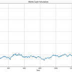
Plot of Monte Carlo Simulation.

plt.plot(monte_carlo_forecast)
plt.xlabel(‘Date’)
plt.ylabel(‘Close At’)
plt.title(‘Monte Carlo Simulation’)
plt.grid(True)
plt.show()

maximun value of the return.

forecast_list[-1:].values.max()

258.1804635163979

minimun value of the return.

forecast_list[-1:].values.min()

13.570891982019532

We respond to several curious queries concerning the stock’s future using the simulation mentioned above.

What is the probability that a stock price will be increased or decreased after 300 days?

We gather the results of each simulation for the following 300th day to respond to this question.

# continous interval frequencies distribution.
x=pd.cut(forecast_list[-1:].values.ravel(),[0,init_val,200]).value_counts()
# reindex.
index_ = [‘Decrease’, ‘Increase’]
x.index=index_
# relative frequencies (Probability of a stock price decrease or increase).
x/len(forecast_list[-1:].values.ravel())

Decrease 0.287671
Increase 0.711029

Bar garph of Probability of a stock price decrease or increase.

ax = plt.figure()
(x/len(forecast_list[-1:].values.ravel())).plot(kind=’bar’,color=[‘red’,’green’])
plt.xticks(rotation=0)
plt.xlabel(‘Stock’)
plt.ylabel(‘Probability’)
plt.title(‘Probability of a stock price decrease or increase’)
plt.ylim(0,1)
plt.grid(axis = ‘y’)

Furthermore, as we can see from the simulation below, the probability of profit increases if we remain in the market for a longer period.

Profit chances plot.

plt.plot(forecast_list)
plt.xlabel('Days')
plt.ylabel('Close At')
plt.title('Monte Carlo Simulation')
plt.axhline(y = init_val, color = 'black', linestyle = '-',linewidth=2.5)
plt.text(5, init_val+5, 'purchase at=51.4 ', fontsize = 22,color='white')
plt.text(299.5, 150, 'Profit', fontsize = 16,color='black')
plt.text(299.5, 30, 'loss', fontsize = 16,color='black')
plt.plot([305,305], [53.5,270],color='green', linestyle = '-',marker = 'o')
plt.plot([305,305], [49,13],color='red', linestyle = '-',marker = 'o')
plt.grid(True)
plt.show()

The above-mentioned machine learning techniques now allow us to answer calls and put in related questions.

Uses cases:

It is possible to predict stock market prices using the GBM model. These Simulations provided answers to a variety of stock price-related queries. Additionally, mention the market risk by the time. so that during a risk occurrence, investors reverse course. Help companies expand their operations and attract investors.

Limitations:

We simulate the behaviour of returns (which are random variables), but we don’t know what factors cause returns. These factors are crucial in determining stock price values.

Feel free to use GitHub code link.