Understanding Temporal Fusion Transformer
Breakdown of Google’s Temporal Fusion Transformer (2021) for interpretable multi-horizon and multivariate time series forecasting.
Temporal Fusion Transformer (TFT) [1] is a powerful model for multi-horizon and multivariate time series forecasting use cases.
TFT predicts the future by taking as input :
- Past target values y within a look-back window of length k
- Time-dependent exogenous input features which are composed of apriori unknown inputs z and known inputs x
- Static covariates s which provide contextual metadata about measured entities that does not depend on time
Instead of just a single value, TFT outputs prediction intervals via quantiles. Each quantile q forecast of τ-step-ahead at time t takes the form:

As an example, to predict future energy consumption in buildings, we can characterize location as a static covariate, weather and data as time-dependent unknown features, and calendar data like holidays, day of week, season, … as time-dependent known features.
Hereafter, an overview of the TFT model architecture:
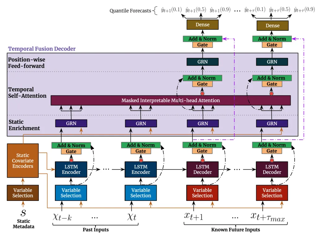
Now let’s dive in each of its blocks!
Gated residual networks
GRN are implemented at different levels of the TFT architecture. They ensure its flexibility by introducing skip/residual connections which feed the output of a particular layer to upper layers in the network that are not directly adjacent.
This way, the model can learn that some non-linear processing layers are unnecessary and skip them. GRN improve the generalization capabilities of the model across different application scenarios (e.g. noisy or small datasets) and helps to significantly reduce the number of needed parameters and operations.

Static covariate encoders
Static covariate encoders learn context vectors from static metadata and inject them at different locations of the TFT network:
- Temporal variable selection
- Local processing of temporal representations in the Sequence-to-Sequence layer
- Static enrichment of temporal representations
This allows to condition temporal representation learning with static information.
Variable selection
A separate variable selection block is implemented for each type of input : static covariates, past inputs (time-dependent known and unknown) and known future inputs.
These blocks learn to weigh the importance of each input feature. This way, the subsequent Sequence-to-Sequence layer will take as input the re-weighted sums of transformed inputs for each time step. Here, transformed inputs refer to learned linear transformations of continuous features and entity embeddings of categorical ones.
The external context vector consists in the output of the static covariate encoder block. It is therefore omitted for the variable selection block of static covariates.

Sequence-to-Sequence
TFT network replaces positional encoding that is found in Transformers [2] by using a Sequence-to-Sequence layer. Such layer is more adapted for time series data, as it allows to capture local temporal patterns via recurrent connections.
Context vectors are used in this block to initialize the cell state and hidden state of the first LSTM unit. They are also employed in what the authors call static enrichment layer to enrich the learned temporal representation from the Sequence-to-Sequence layer with static information.
Interpretable Multi-head attention
Attention mechanism weighs the importance of values based on the relationships between keys and queries. This is by analogy with information retrieval that would evaluate a search query (query) against document embeddings (keys) to retrieve most relevant documents (values).

where α(Q,K) are attention weights. A common choice for α is the scaled dot-product attention.
Original multi-attention mechanism, proposed in [2], consists in using multiple attention heads to re-weigh the values based on the relevance between keys and queries. The outputs of different heads are then combined via concatenation, as follows :

where W_H, W_Q, W_K, W_V are projection weight matrices and h is the number of attention heads.
In self-attention, queries, keys and values come from the same input. This allows to learn the relevance of each time step with respect to the rest of the input sequence, and therefore to capture long-range temporal dependencies. Note that at the decoder part, subsequent time steps at each decoding step are masked to avoid information leakage from future to past data points.
TFT adjusts this definition to ensure interpretability. As such, instead of having multiple head-specific weights for values, these are shared across all attention heads. This allows to easily trace back most relevant values. The outputs of all heads are then additively aggregated :


Quantile regression
Instead of just a single value, TFT predicts quantiles of the distribution of target ŷ using a special quantile loss function, also known as pinball loss :

Intuitively, the first term of this loss function is activated for under-estimations and is highly weighted for upper quantiles, whereas the second term is activated for over-estimations and is highly weighted for lower quantiles. This way, the optimization process is forcing the model to provide reasonable over-estimations for upper quantiles and under-estimations for lower quantiles. Notice that for the median prediction (0.5 quantile), optimizing quantile loss function is equivalent to that of the MAE loss.
TFT is then trained by minimizing an aggregate of all quantile losses across all quantile outputs.
Quantile regression is very useful for high-stakes applications to have some kind of a quantification of uncertainty of predicted values at each time step.
Interpretability
As discussed in earlier sections, TFT enables a new form of interpretability via:
- Variable selection blocks that explicitly learn global importance weights of input features
- Adjusting the standard multi-head attention definition to have shared weights for values across all attention heads
Interpretable attention weights are useful for 2 cases :
- Easily trace back most relevant past time-steps to predict each forecast. Such insight is traditionally gained using preliminary seasonality and autocorrelation analysis
- Identify significant changes in temporal patterns. This is done by computing an average attention pattern per forecast horizon and evaluate the distance between it and attention weights at each point.
Existing implementations
Some available TFT model implementations are:
- Pytorch Forecasting : https://pytorch-forecasting.readthedocs.io/en/stable/tutorials/stallion.html
- Darts : (adopted from Pytorch Forecasting implementation) https://unit8co.github.io/darts/examples/13-TFT-examples.html?highlight=temporal%20fusion
Both implementations are based on Pytorch Lightning.
You can refer to this blog post about using TFT for book sales forecasting:
Key Takeaways
TFT is a transformer for time series data. It supports:
- Multi-horizon forecasting
- Multivariate time series with heterogeneous features (support for static covariates, time varying known and unknown variables)
- Prediction intervals to quantify uncertainty
- Interpretablity of results
TFT is mainly able (1) to capture temporal dependencies at different time scales by a combination of the LSTM Sequence-to-Sequence and the Transformer’s Self-Attention mechanism, and (2) to enrich learned temporal representations with static information about measured entities.
Thank you for reading!
References
[3] Yasuto Tamura, Multi-head attention mechanism, https://data-science-blog.com/blog/2021/04/07/multi-head-attention-mechanism/