Is grid trading more profitable than liquidity provision?

This is a guest post by Omer Arbnom Yanar, an independent researcher. He expressed his opinions about grid trading in this article, which may not represent the views of DeGate DAO. You can do grid trading on DeGate, with zero trading fees

In today’s financial world, there are many trading strategies catering to different risk levels of traders. Some strategies need traders to be fully involved, while others can run on their own. Grid trading is a strategy that’s easy to automate.

In this post, we will discuss the main aspects of grid trading and compare grid trading positions and concentrated liquidity positions, both theoretically and based on past price data. Here is the content list:

• What is Grid Trading?
• Similarities and Differences with Concentrated Liquidity Positions
• Impermanent Loss and Profit Scenarios
• Modeling a Grid Trading Setup with -1,1 Sequences
• A PnL Calculation Example with the -1,1 Sequence
• Analyzing -1,1 Sequences with Python
• Backtesting Grid Trading Positions with Python
• Comparison of Grid Trading and Concentrated Liquidity Positions
• Conclusion

What is Grid Trading?

The basic idea of grid trading is to set up a grid on the price chart and make buy and sell orders based on that grid. There are two main ways to do grid trading. The first is called against-the-trend grid trading. In this method, you place buy and sell orders against the current trend. This approach involves selling as prices rise and buying as they fall. This works well when prices move up and down within a certain range, letting you buy at low prices and sell at high prices. The second method is called with-the-trend grid trading. In this approach, you make orders that follow the trend. When the price is going up, you keep buying, which increases your investment. And when the price goes down, you start selling. This method creates large trend-following positions, requiring timely actions to secure profits when trends change. This makes it harder to fully automate. In this post, we’ll focus on the against-the-trend method, which we’ll just call normal grid trading.

To better understand normal grid trading, let’s look at an example. Imagine we have a setup with 6 grids between $1300 and $1306. When the price hits a grid from below, it triggers a sell order, and that grid becomes a new waiting line. At the same time, a new buy order is placed at the previous waiting line. And if the price hits a grid from above, a buy order is triggered, setting a new waiting line where a sell order is then placed at the previous waiting line.

The quantity per grid refers to how much of an asset is traded with each movement through the grid. For example, trading 1 ETH per grid, Alice would need an initial 3 ETH and 3903 USDC (summing up 1302, 1301, and 1300 for each grid) to establish her grid trading setup. By setting up this grid, Alice sees a profit of 3 USDC due to price movements.

Similarities and Differences with Concentrated Liquidity Positions

Grid trading shares similarities with providing concentrated liquidity in an AMM pool, like Uniswap V3, where positions are set within a specific range. This similarity holds from the perspective of both DEXs and users.

From the DEXs’ viewpoint, adding liquidity to an AMM pool enhances swap efficiency by reducing slippage, thanks to the X*Y=K formula. Similarly, establishing a grid trading position adds liquidity at each grid point through the placed limit orders, aiding efficient swaps for market participants.

For users’ perspective, both strategies offer profit-making opportunities through the trades conducted within their set range. Liquidity provision in a pool generates fees from all swaps within that range, whereas grid trading profits come from price movements across the grid levels. Both methods, however, are susceptible to impermanent loss. This is because they involve selling assets as prices rise and buying as they fall, which could lead to the total value of the positions being lower than simply holding the assets. Yet, if prices return to their starting point, the loss from price changes is nullified, and profits are realized. However, there’s no guarantee prices will revert, so position holders must be proactive in managing potential losses.

Both liquidity providers and grid traders are at risk of impermanent loss, but the extent of the loss isn’t identical. Suppose Alice sets up a liquidity position and Bob employs a grid trading strategy within the same price range and with equal investments. In this case, Bob is likely to incur a smaller impermanent loss. This is because, as prices rise, liquidity providers like Alice are selling their assets at every incremental price change, whereas grid traders like Bob wait for specific price points to execute their sales. Similarly, as prices drop, Alice continuously buys back, but Bob waits for predetermined prices to make his purchases. This strategic difference is why grid traders typically face less impermanent loss compared to liquidity providers when starting under similar conditions.

Furthermore, the drivers of profit for both types of position holders diverge significantly. For liquidity providers, trading volume is crucial for generating fee income. In contrast, for grid traders like Bob, volume is less impactful; their profits hinge on price oscillations within the grid that enable buying low and selling high.

However, optimizing the grid sizes and price range is not straightforward. Increasing the number of grids can lead to more trades, but also it may reduce the profit per grid due to decreased trade sizes and narrower grid widths. Moreover, without price oscillation, an increased number of transactions can result in higher average costs. For instance, purchasing 1 ETH at $2200 outright is more cost-effective than buying 0.5 ETH at $2250 and another 0.5 ETH at $2200. Conversely, if the price is oscillating around $2200–2250 the strategy containing more grids gives better results. Consequently, the optimal grid setup heavily relies on prevailing market conditions. It’s also worth noting that maker fees play a role, although many order book DEXs do not charge maker fees.

Impermanent Loss and Profit Scenarios

Now, let’s talk about risks and potential losses. Imagine the ETH price is $2500, and Alice sets up a grid trading range between $2000 and $3000, consisting of 100 grids, each with a 0.1 ETH quantity. To place sell orders, she needs 5 ETH (50*0.1) and for buy orders, she requires 11225 USDC, calculated as 0.1(2490+2480+…+2010+2000). Suppose Alice sets stop-loss orders at $3000.01 and $1999.99 to limit losses if the price moves out of her range. The primary risk she faces within the $2000-$3000 range is impermanent loss.

Before we dive into the calculations, let’s understand what impermanent loss is. Assume the price rises to $2800, filling 30 of her sell orders, meaning she sells 0.1 ETH at prices ranging from 2510 to 2800. As a result, she gains 7965 USDC in exchange for 3 ETH (0.1*30). So, she sold her 3 ETH for $7965. Given the current price is $2800, she incurs a loss of $435 (3*2800–7965).

To generalize the concept of impermanent loss with Alice’s grid trading strategy, consider her series of sell orders within a price range of $2510 to $2800, spanning 29 grids. If Alice had refrained from selling 0.1 ETH at the initial grid price of $2510 and instead waited to sell at $2800, she would have realized a profit of $29, calculated as 29*(10*0.1). This missed profit represents the impermanent loss from her first sale, amounting to $29. As Alice continues to sell at each subsequent grid, the impermanent loss from each sale decreases incrementally by $1, culminating in a total impermanent loss of $435 across all sales, with the calculation following the sequence 29+28+27+…+2+1. It’s important to note that the final sale does not contribute to the impermanent loss, underscoring that this loss diminishes with each grid passed. This principle holds true regardless of the price direction, ensuring symmetry in the calculation for both positive and negative price movements.

To generalize further, let ‘d’ represent the difference between grid prices, and ‘q’ the quantity per grid. If the price moves ’n’ grids from the starting point, the current impermanent loss is dq(1+2+…+n-1) = dq(n-1)n/2. Thus, if the furthest grid from the starting point is ‘m’ grids away, the maximum loss would be dq*(m-1)m/2. In the example given, with ‘d’ being 10, ‘q’ 0.1, and ‘m’ 50, the maximum impermanent loss Alice could face, with stop-loss orders in place, is 100.104950/2 = $1225.

Now, let’s consider profits in a scenario where prices move randomly. Before modeling random price movements, it’s important to note that if a sell order is executed right after a buy order, Alice realizes a profit of $d*q, given that ‘d’ the difference between grids and ‘q’ is the quantity per grid. This also holds if a buy order precedes a sell order. What if these pairs are not consecutive, for example, if several buy orders are triggered by a downtrend? Without a price reversal allowing Alice to sell the assets she bought, she faces impermanent loss. However, if prices revert, she essentially sells each purchased asset at one grid higher, mitigating loss. This principle applies to uptrends as well. The illustration below demonstrates how buy and sell points are matched.

Modeling a Grid Trading Setup with -1,1 Sequences

Also, note that the price movement between grids is not crucial for us, as no transactions occur in these areas. Our focus is solely on the grids impacted by the price changes. Let’s develop a simplified model for random price movements. For ease of understanding, we’ll assume an even number of grids with the starting position at the center, balancing buy and sell orders. This model can be adapted for asymmetrical starting positions. In this setup, if the price reaches a grid from below, Alice sells the asset; if it comes from above, she buys. Since our interest lies in the direction of price changes and the specific grid levels affected, we can summarize the price movements using a sequence of -1 and 1. The sequence’s length corresponds to the number of grids the price touches. To construct this sequence, we observe the price movement: a move to the first grid above the starting point is marked as 1, and a move to a lower grid is marked as -1. This method allows us to encapsulate the price dynamics in a sequence of -1 and 1, simplifying our analysis. Let’s revisit our earlier example to illustrate this.

In this scenario, six grids are reached, so the sequence will consist of six elements. Our sequence, representing these movements, will be [-1, 1, 1, -1, -1, 1].

When we use a series of -1 and 1 to represent positions, an important factor to consider is the range. Some sequences may suggest price movements that extend beyond our designated range. To identify such occurrences, we need to examine the cumulative sums of the sequence. This allows us to track each grid crossed by the price change. For instance, consider the partial sum of the sequence [1, 1, -1, -1, -1, 1, 1, 1, -1, -1, 1, -1, 1, -1, 1, 1, -1, 1]. The nth term of the partial sum is the sum of the first n terms of the original sequence. In this case, the cumulative sum is [1, 2, 1, 0, -1, 0, 1, 2, 1, 0, 1, 0, 1, 0, 1, 2, 1, 2], indicating that the price fluctuates within a range of two grids below and three grids above the starting point.

A PnL Calculation Example with the -1,1 Sequence

It’s clear that any price movement can be represented by a sequence for a given grid setup. Although a single sequence may correspond to multiple price movements, this does not concern us as our focus is solely on the grids reached by the price. Thus, by analyzing the sequence, we can predict every possible outcome of grid setup and price movement. Let’s explore how to calculate the profit and loss (PnL) for a position based on its sequence. To maintain consistency, we’ll use Alice’s setup as an example. The initial price is set at $2500, within a range of $2000 to $3000, distributed across 100 grids. Each grid holds a quantity of 0.1 ETH, and the initial balance consists of 5 ETH and $11225 USDC.

Consider a series of -1 and 1, like [1, 1, -1, -1, -1, 1, 1, 1, -1, -1, 1, -1, 1, -1, 1, 1, -1, 1], with 18 terms where 10 are 1s and 8 are -1s. By pairing up the 1s and -1s, we’re left with two unpaired 1s, indicating 8 completed transactions and a final price 2 grids above the starting point. Given each grid represents a $10 change and Alice trades 0.1 ETH per grid, she earns $1 for each transaction, totaling $8 in profit.

To calculate the profit and loss (PnL), let’s start with Alice’s initial assets: 5 ETH and 11225 USDC at a $2500 ETH price, totaling $23725. If the final price is 2 grids higher, between $2520 and $2530, let’s assume $2520. Having sold 0.2 ETH, her final assets are 4.8 ETH and 11728 USDC, valuing her position at $23824, plus the $8 transaction profit, summing up to $23832. Therefore, her PnL from the strategy is $107.

Considering impermanent loss, had Alice simply held her initial assets, her value at a $2520 ETH price would be $23825. Thus, her strategy incurs a $1 impermanent loss compared to a $100 profit from holding, leading to a net gain of $99 from price movements and $8 from transactions, making her strategy 7% more profitable than merely holding.

Analyzing -1,1 Sequences with Python

The example above illustrates how a grid trading strategy can outperform simple holding, although this isn’t always the case. To explore various scenarios, I’ve prepared a GitHub repository (https://github.com/arbnom/Grid-Trading-Strategy-Analysis) with three Python scripts that consider stop-loss orders outside the price range, offering insights into different trading outcomes.

The first script, “longest_valid_subsequence_result.py,” analyzes a given position with parameters such as the -1,1 sequence, initial grid position, number of grids, quantity per grid, and distance between grids. It first checks if the price exits the range; if it does, the script identifies the longest subsequence within the range. It then calculates the sequence’s length and sum, followed by the impermanent loss based on the sum and realized profit from the -1,1 pairs. The outcome represents the difference between realized profit and impermanent loss, providing a comparison between holding and employing a grid strategy rather than the position’s profit and loss (PnL). To determine the PnL, we must incorporate price data, which we will address shortly.

“longest_valid_subsequence_result.py” specifically evaluates a singular position’s outcome. For broader analysis, we require additional data. The term “expectation” refers to the weighted average of outcomes, with the weights being the probabilities of those outcomes. For instance, in a game where rolling a fair six-sided die earns the roller an equivalent amount of ETH, the expected outcome is 3.5 ETH, indicating the average earnings if the game is played numerous times.

The second and third scripts calculate the expectation for a random grid trading position, taking inputs like the number of grids, hit grids, quantity per grid, and distance between grids. “average_sequence_upto_length.py” generates all sequences within the range and up to the specified length, analyzing their outcomes compared to holding and averaging the results. “average_sequence_fixed_length.py” performs a similar function but focuses on sequences of a fixed length, providing a thorough examination of strategy outcomes against holding.

These tools are helpful when we know the grid setup and the sequence length of the price changes, allowing us to estimate the expected outcome for a trading strategy under various market conditions. However, they simplify market dynamics by assuming each scenario is equally probable, neglecting trend behaviors. Despite this limitation, these methods can uncover valuable insights.

For instance, if the sequence length surpasses the number of grids, the expected outcome consistently turns positive. This happens because the potential impermanent loss is confined by the grid number, computed as dq(n-1)n/2, where d is the grid gap, q is the quantity per grid, and n is the number of grids from the starting position to the end position. Since the maximum step count from the start is the grid number, and the realized profit equals dq(L-n)/2 for a sequence of length L, extending the sequence length while maintaining the grid count boosts the realized profits.

Another intriguing point is that the expected outcome zeroes out if the sequence length is at or below the grid count, a fact provable through combinatorics. For a sequence of length k, the possible steps from the starting position are k, k-2, k-4, k-6, etc. This principle applies to both “average_sequence_fixed_length.py” and “average_sequence_upto_length.py.”

Thus, letting the price hit more grids than the total grid count shifts the expected outcome from neutral to positive, advantageous for the trader assuming market movements are random. However, calculating the longer the sequence, the higher the computational demand due to the increase in possible sequences.

Backtesting Grid Trading Positions with Python

Let’s explore how to calculate the Profit and Loss (PnL). I’ve set up a GitHub repository that enables backtesting strategies based on historical data, available at https://github.com/arbnom/Grid-Trading-Backtest-Tool. To compute the PnL of a position, we need details such as price history, price range, grid count, quantity per grid, and the duration the position was held. The repository includes two sections: one for strategies with a stop-loss condition and another without.

Focusing on the codes with stop-loss, we start with “calc_of_grids.py,” which determines the grid values based on the grid range and count. This step sets the foundation. Next, we generate the -1,1 sequence reflecting the price movements against these grid values.

“generate_with_stoploss.py” first outlines the grid ranges. Using price data, it then crafts a -1,1 sequence by marking a ‘1’ when the price reaches a higher grid and ‘-1’ when it dips below a grid. The sequence generation halts if the price exits the predefined range. In contrast, the counterpart code without stop-loss waits for the price to re-enter the range before continuing the sequence. Finally, it estimates the initial assets needed by considering the planned orders and the quantity per grid.

This approach provides a structured method to analyze the potential outcomes of grid trading strategies, taking into account the fluctuations within a specified price range and applying a stop-loss strategy to mitigate risk.

Once we have the -1,1 sequence, calculating the PnL becomes straightforward. The script “result_with_stoploss.py” first determines the initial value of the position using the starting amounts of assets and the initial price. It then updates the ETH and USDC values after each trade, corresponding to each element in the sequence. Utilizing the sequence and grid values, the script also calculates the final ETH price, simplifying the process of determining the position’s final value. The PnL is the difference between the final and initial values. For a more comprehensive analysis, the script also computes the impermanent loss and the realized profit.

Additionally, we have a diagnostic script named “debug_with_stoploss.py” that performs the same calculations as “result_with_stoploss.py” but also outputs each step. This feature is particularly useful for identifying and resolving any issues that may arise.

The data used in these analyses is sourced from TradingView and pertains to the ETH/USDC pair on Binance, spanning from 2024–01–22T00:00:00Z to 2024–02–07T15:49:00Z. To update the dataset, start with the new data from 2024–02–07T15:45:00Z, formatted as time, open, high, low, close, volume, and volume MA. I averaged the high and low prices for each minute. To transform this data into the required format, you can use Python or another programming language. With GPT-4, you can input the data directly, and it will generate the desired CSV file.

Comparison of Grid Trading and Concentrated Liquidity Positions

Being a liquidity provider on Uniswap V3 is akin to managing a grid trading position. Having developed a tool for backtesting grid trading strategies, we can now compare its performance with that of Uniswap V3. To acquire Uniswap data, I utilized Revert Finance. A minor drawback of Revert Finance is that it updates data hourly, whereas our CSV file contains minute-by-minute price information. However, this discrepancy becomes negligible over longer analysis periods.

Before we dive into comparisons, it’s important to set our expectations. Uniswap V3’s efficiency improves as the range narrows, assuming the price remains within this range. Narrower ranges mean more of the provided liquidity is utilized for trades, generating fee income. Conversely, the performance of a grid trading position depends on the number of realized profits, the distance between grids, and the quantity per grid. Narrowing the range could negatively impact grid trading positions by reducing the distance between grids and the quantity per grid, even if it increases the number of realized profits. However, we cannot generalize these observations, as UniV3’s efficiency is significantly influenced by trading volume. If the volume is notably low, holding positions within a tight range may yield as much profit as a broader position with high volume. Similarly, the performance of grid trading is closely tied to price fluctuations. If the market doesn’t fluctuate sufficiently — evidenced by a short -1,1 sequence — the spacing between grids and the quantity per grid may have little to no impact on the PnL.

To compare Uniswap V3 and grid trading, I’ve considered four different durations: 14 days, 7 days, 48 hours, and 24 hours, with three range types for each: safe, neutral, and aggressive. Safe ranges ensure the price always stays within the range, neutral ranges see the price occasionally move outside, and aggressive ranges are so narrow that the price often falls outside. Given the nature of these strategies, it’s challenging to align the initial amounts exactly, but I’ve managed to keep them within a 0.03% difference, meaning if one position starts with $50,000, the other’s initial value ranges between $49,985 and $50,015.

I’ll first present a table comparing only the PnLs, with detailed position information provided at the end of the post. Let’s take a look at the PnL comparison table.

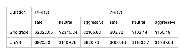
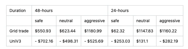
In the analysis above, it’s clear that grid trading generally outperformed in the durations examined, suggesting that price movements played a more significant role than trading volume during these periods. However, this data alone isn’t sufficient to conclude that grid trading is superior overall. The seven-week analysis highlights how Uniswap V3 can excel when set to ranges of high volume. From this, one might deduce that Uniswap V3 tends to yield better results if one can accurately predict high-volume ranges; otherwise, a grid trading strategy is a viable alternative.

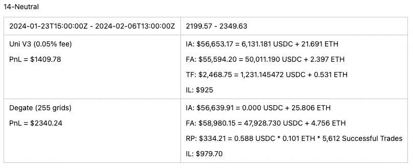
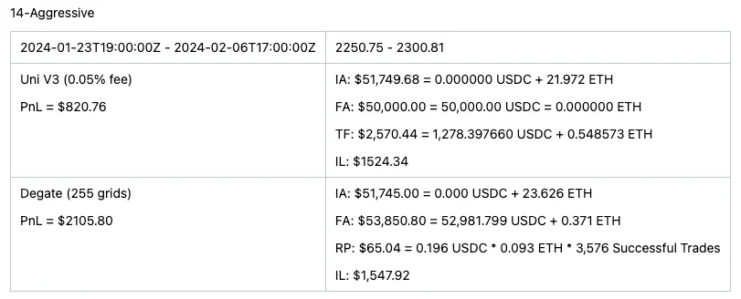
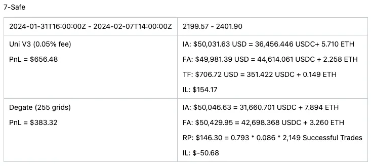
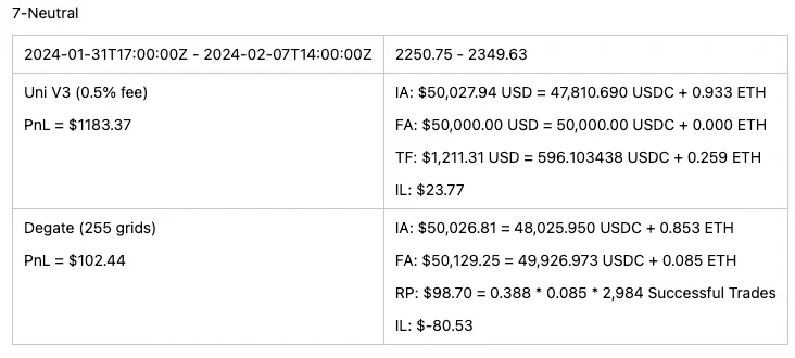
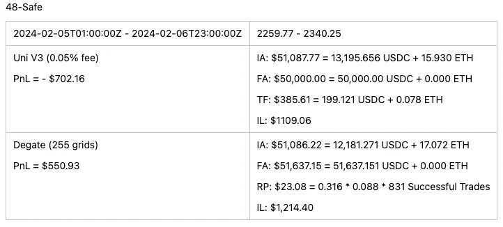
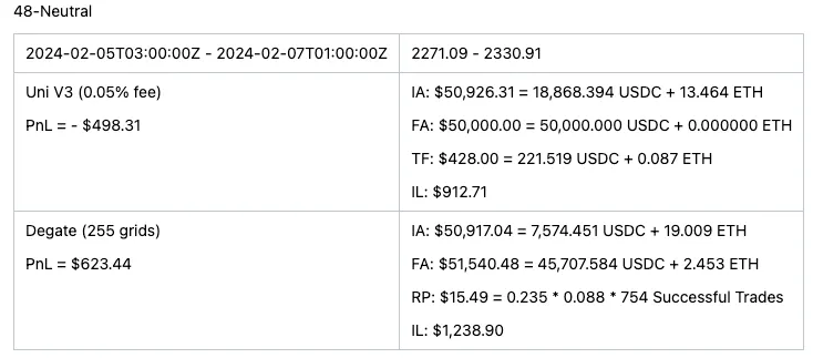
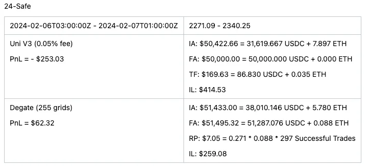
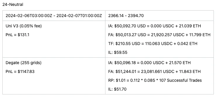
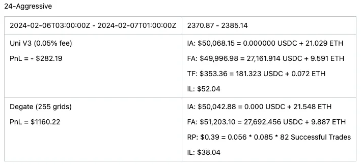
For those keen on a deeper dive into the comparison, I’m providing detailed breakdowns of both strategies. It’s crucial to note that Revert Finance calculates impermanent loss based on the USD value change from initial to final amounts. Yet, a precise assessment of impermanent loss requires comparing the initial asset amounts’ current value to the final amount. Hence, in the following tables, impermanent loss has been recalculated accurately.

The tables use abbreviations where “IA” stands for initial amount, “FA” for final amount, “TF” for total generated fees, “IL” for impermanent loss, and “RP” for realized profit.

This analysis offers a nuanced view of grid trading and Uniswap V3 strategies, considering their dependency on market dynamics like volume and price fluctuations. The provided tables aim to facilitate a comprehensive comparison, incorporating corrections for accurately measuring impermanent loss.

14-Safe

14-Neutral

14-Aggressive

7-Safe

7-Neutral

7-Aggressive

48-Safe

48-Neutral

48-Aggressive

24-Safe

24-Neutral

24-Aggressive

Conclusion

Wrapping up, we’ve looked at grid trading from top to bottom, compared it to concentrated liquidity like in Uniswap V3, and used past price data to see how they stack up. We found that grid trading can work well, especially when prices keep moving up and down. But it’s not always the best choice. Our seven-week study showed that Uniswap V3 can do better when there’s a lot of trading going on.

So, what’s the main point? It’s that both grid trading and concentrated liquidity can be successful. It all comes down to the market’s behavior. If you’re good at predicting when there’ll be lots of trading, Uniswap V3 might be better. But if the market’s bouncing around a lot, then grid trading could be the way to go.

In the end, it’s all about forecasting the market and picking the strategy that fits best with what’s happening. This post should give you a good start on figuring out which strategy to use and when.