Option Greeks and Hedging Strategies
The aims of the actual research are, firstly, to present some of the most efficient methods to hedge option positions and, secondly, to show how important option Greeks are in volatility trading. It is worth mentioning that the present study has been completely developed by Liying Zhao (Quantitative Analyst at HyperVolatility) and all the simulations have been performed via the HyperVolatility Option Tool–Box. If you are interested in learning about the fundamentals of the various option Greeks please read the following studies “Options Greeks: Delta, Gamma, Vega, Theta, Rho” and “Options Greeks: Vega, Charm, Vomma, DvegaDtime”.
In this research, we will assume that the implied volatilityσis not stochastic, which means that volatility is neither a function of time nor a function of the underlying price. As a practical matter, this is not true, since volatility constantly change over time and can hardly be explicitly forecasted. However, doing researches under the static–volatility framework, namely, the Generalized Black–Scholes–Merton (GBSM) framework, we can easily grasp the basic theories and then naturally extend them to stochastic volatility models.
Recall that the Generalized Black–Scholes–Merton formula for pricing European options is:
C = Se (b-r)T N(d1) — Xe -rT N(d2)
P = Xe -rT N(–d2) — Se (b-r)T N(–d1)
Where


And N ( ) is the cumulative distribution function of the univariate standard normal distribution. C = Call Price, P = Put Price, S = Underlying Price, X = Strike Price, T = Time to Maturity, r = Risk–free Interest Rate, b = Cost of Carry Rate, σ= Implied Volatility.
Accordingly, first order GBSM option Greeks can be defined as sensitivities of the option price to one unit change in the input variables. Consequentially, second or third–order Greeks are the sensitivities of first or second–order Greeks to unit movements in various inputs. They can also be treated as various dimensions of risk exposures in an option position.
1. Risk Exposures
Differently from other papers on volatility trading, we will initially look at the Vega exposure of an option position.
1.1 Vega Exposure
Some of the variables in the option pricing formula, including the underlying price S, risk–free interest rate r and cost of carry rate b, can be directly collected from market sources. Strike price X and time to maturity T are agreed with the counterparties. However, the implied volatility σ, which is the market expectation towards the magnitude of the future underlying price fluctuations, cannot be explicitly derived from any market source. Hence, a number of trading opportunities arise. Likewise directional trading, if a trader believes that the future volatility will rise she should buy it while, if she has a downward bias on future volatility, she should sell it. How can a trader buy or sell volatility?
We already know that Vega measures option’s sensitivity to small movements in the implied volatility and it is identical and positive for both call and put options, therefore, a rise in volatility will lead to an increase in the option value and vice versa. As a result, options on the same underlying asset with the same strike price and expiry date may be priced differently by each trader since everyone can input her own implied volatility into the BSM pricing formula. Therefore, trading volatility could be, for simplicity, achieved by simply buying under–priced or selling over–priced options. For finding out if your implied volatility is higher or lower than the market one, you can refer to this research that we previously posted.
Let’s assume an option trader is holding a so–called ‘naked’ short option position, where she has sold 1,000 out–of–the–money (OTM) call options priced with S=$90, X=$100, T=30 days, r=0.5%, b=0, σ=30%, which is currently valued at $434.3. Suppose the market agreed implied volatility decreases to 20%, other things being equal, the option position is now valued at $70.6. Clearly, there is a mark–to–market profit of $363.7 (434.3–70.6) for this trader. This is a typical example of Vega exposure.
Figure 1 shows the Vega exposure of above the option position. It can be easily observed that the Vega exposure may augment or erode the position value in a non–linear manner:

(Figure 1. Source: HyperVolatility Option Tool — Box)
A trader can achieve a given Vega exposure by buying or selling options and can make a profit from a better volatility forecast. However, the value of an option is not affected solely by the implied volatility because when exposed to Vega risk, the trader will simultaneously be exposed to other types of risks.
1.2 Theta Exposure
Theta is the change in option price with respect to the passage of time. It is also called ‘time decay’ because Theta is considered to be ‘always’ negative for long option positions. Given that all other variables are constants, option value declines over time, so Theta can be generally referred to as the ‘price’ one has to pay when buying options or the ‘reward’ one receives from selling options. However, this is not always true. It is worth noting that some researchers have reported that Theta can be positive for deep ITM put options on non–dividend–paying stocks. Nevertheless, according to our research, which is displayed in Figure 2, where X=$100, T=30 days, r=0.5%, b=0, σ =30%, the condition for positive Theta is not that rigorous:
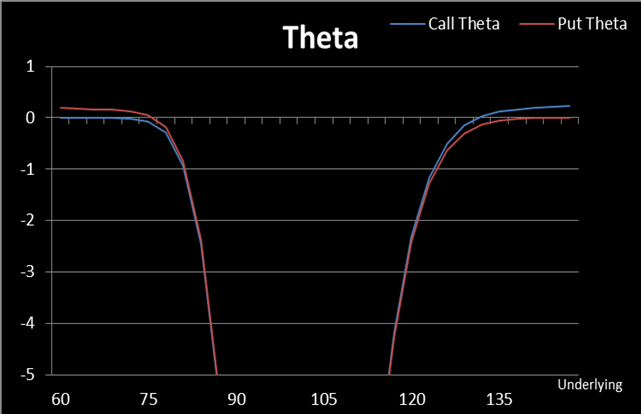
(Figure 2. Source: HyperVolatility Option Tool — Box)
For deep in–the–money (ITM) options (with no other restrictions) Theta can be slightly greater than 0. In this case, Theta cannot be called ‘time decay’ any longer because the time passage, instead, adds value to bought options. This could be thought of as the compensation for option buyers who decide to ‘give up’ the opportunity to invest the premiums in risk–free assets.
Regarding the aforementioned instance, if an option trader has sold 1,000 OTM call options priced with S=$90, X=$100, T=30 days, r=0.5%, b=0, σ=30%, the Theta exposure of her option position will be shaped like in Figure 3:
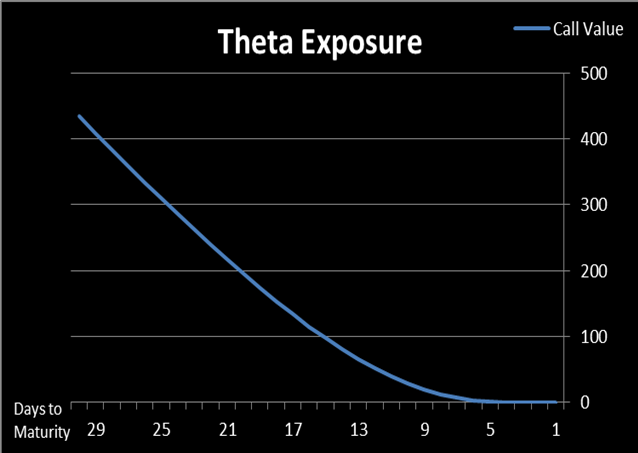
(Figure 3. Source: HyperVolatility Option Tool — Box)
In the real world, none can stop time from elapsing so Theta risk is foreseeable and can hardly be neutralized. We should take Theta exposure into account but do not need to hedge it.
1.3 Interest Rate/Cost of Carry Exposure (Rho/Cost of Carry Rho)
The cost of carry rate b is equal to 0 for options on commodity futures and equals r–q for options on other underlying assets (for currency options, r is the risk–free interest rate of the domestic currency while q is the foreign currency’s interest rate; for stock options, r is the risk–free interest rate and q is the proportional dividend rate). The existence of r, q and b does have an influence on the value of the option. However, these variables are relatively determinated in a given period of time and their change in value has rather insignificant effects on the option price. Consequently, we will not go too deep into these parameters.
1.4 Delta Exposure
Delta is the sensitivity of the option price with regard to changes in the underlying price. If we recall the aforementioned scenario (where a trader has sold 1,000 OTM call options priced with S=$90, X=$100, T=30 days, r=0.5%, b=0, σ =30%, valued at $434.3) if the underlying price moves downwards, the position can still be able to make profits because the options will have no intrinsic value and the seller can keep the premiums. However, if the underlying asset is traded at, say, $105, all other things being equal, the option value becomes $6,563.7, which leads to a notable mark–to–market loss of $6,129.4 (6,563.7–434.3) for the option writer. This is a typical example of Delta risk one has to face when trading volatility. Figure 4 depicts the Delta exposure of the above mentioned option position, where we can see that the change in the underlying asset price has significant influences on the value of an option position:
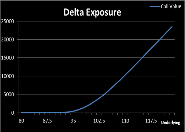
(Figure 4. Source: HyperVolatility Option Tool — Box)
Compared to Theta, Rho and cost of carry exposures, Delta risk is definitely much more dominating in volatility trading and it should be hedged in order to isolate volatility exposure. Consequentially, the rest of this paper will focus on the introduction to various approaches for hedging the risk with respect to the movements of the underlying price.
2. Hedging Methods
At the beginning of this section, we should clearly define two confusable terms: hedging costs and transaction costs. Generally, hedging costs could consist of transaction costs and the losses caused by ‘buy high’ and ‘sell low’ transactions. Transaction costs can be broken down into commissions (paid to brokers, etc.) and the bid/ask spread. These two terms are usually confounded because both of them have positive relationships with hedging frequency. Mixing these two terms up may be acceptable, but we should keep them clear in mind.
2.1 ‘Covered’ Positions
A ‘covered’ position is a static hedging method. To illustrate it, let us assume that an option trader has sold 1,000 OTM call options priced with S=$90, X=$100, T=30 days, r=0.5%, b=0, σ=30%, and has gained $434.3 premium. Compared to the ‘naked’ position, this time, these options are sold simultaneously with some purchased underlying assets, say, 1,000 stocks at $90. In this case, if the stock price increases to a value above strike price (e.g. $105) at maturity, the counterparty will have the motivation to exercise these options at $100. Since the option writer has enough amount of stocks on hand to meet the exercise demand, ignoring any commission, she can still get a net profit of 1,000*(100–90) + 434.3= $10,434.3. On the contrary, if the stock price stays under the strike price (e.g. $85) upon expiry date, the seller’s premium is safe but has to suffer a loss in stock position which in total makes the trader a negative ‘profit’ of 1,000*(85–90) + 434.4=-$4565.7. The ‘covered’ position can offer some degrees of protection but also induces extra risks in the meantime. Thus, it is not a desirable hedging method.
2.2 ‘Stop-Loss’ Strategy
To avoid the risks incurred by stock prices’ downward trends in the previous instance the option seller could defer the purchase of stocks and monitor the movements of the stock market. If the stock price is higher than the strike price, 1,000 stocks will be bought as soon as possible and the trader will keep this position until the stock price will fall below the strike. This strategy seems like a combination of a ‘covered’ position and a ‘naked’ position, where the trader is ‘naked’ when the position is safe and he is ‘covered’ when the position is risky.
The ‘stop-loss’ strategy provides some degrees of guarantee for the trader to make profits from option position, regardless of the movements of the stock price. However, in reality, since this strategy involves ‘buy high’ and ‘sell low’ types of transactions, it can induce considerable hedging costs if the stock price fluctuates around the strike.
2.3 Delta–Hedging
A smarter method to hedge the risks from the movements of the underlying price is to directly link the amount of bought (sold) underlying asset to the Delta value of the option position in order to form a Delta– neutral portfolio. This approach is referred to as Delta hedging. How to set up a Delta–neutral position?
Again, if a trader has sold 1,000 call options priced with S=$90, X=$100, T=30 days, r=0.5%, b=0, σ=30% the Delta of her position will be -$119 (-1,000*0.119), which means that if the underlying increases by $1, the value of this position will accordingly decrease by $119. In order to offset this loss, the trader can buy 119 units of underlying, say, stocks. This stock position will give the trader $119 profit if the underlying increases by $1. On the other hand, if the stock price decreases by $1, the loss on the stock position will then be covered by the gain in the option position. This combined position seems to make the trader immunized to the movements of the underlying price.
However, in the case the underlying trades at $91, we can estimate that the new position Delta will be -$146. Obviously, 119 units of stocks can no longer offer full protection to the option position. As a result, the trader should rebalance her position by buying 27 more stocks to make it Delta–neutral again.
By doing this continuously, the trader can have her option position well protected and will enjoy the profit deriving from an improved volatility forecasting. Nevertheless, it should be noted that Delta–hedging also involves ‘buy high’ and ‘sell low’ operations which could cause a loss for every transaction related to the stock position. If the price of the underlying is considerably volatile, the Delta of the option position would change frequently, meaning the option trader has to adjust her stock position accordingly with a very high frequency. As a result, the cumulative hedging costs can reach an unaffordable level within a short period of time.
The aforementioned instance show that increasing hedge frequency is effective for eliminating Delta exposure but counterproductive as long as hedging costs are concerned. To reach a compromise between hedge frequency and hedging costs, the following strategies can be taken into considerations.
2.4 Delta–Gamma Hedging
In the last section, we have found that Delta hedging needs to be rebalanced along with the movements of the underlying. In fact, if we can make our Delta immune to changes in the underlying price, we would not need to re–hedge. Gamma hedging techniques can help us accomplishing this goal (recall that Gamma is the speed at which the Delta changes with respect to movements in the underlying price).
The previously reported example, where a trader has sold 1,000 call options priced with S=$90,X=$100,T=30days,r=0.5%,b=0 ,
σ =30% had a position Delta equal to -$119 and a Gamma of -$26. In order to make this position Gamma–neutral, the trader needs to buy some options that can offer a Gamma of $26. This can be easily done by buying 1,000 call or put options priced with the same parameters as the sold options. However, buying 1,000 call options would erode all the premiums the trader has gained while buying 1,000 put options would cost the trader more, since put options would be much more expensive in this instance. A positive net premium can be achieved by finding some cheaper options.
Let us assume that the trader has decided to choose, as a hedging tool, the call option priced with S=$90, X=$110, T=30 days, r=0.5%, b=0, σ=30%, with 0.011 Delta and 0.00374 Gamma. To offset his sold Gamma, the trader needs to buy 26/0.00374 = 6,952 units of this option which cost him $197.3 which leads to an extra Delta of 6,952*0.011=$76. At this point, the trader has a Gamma–neutral position with a net premium of $237 (434.3–197.3) and a new Delta of -$43(-119+76). Therefore, buying 43 units of underlying will provide the trader with Delta neutrality. Now, let’s suppose that the underlying trades at $91, the Delta of this position would become -$32 but since the trader had already purchased 43 units of stocks, she only needs to sell 12 units to make this position Delta–neutral. This is definitely a better practice than buying 27 units of stocks as explained in section 2.3 where the trader had only Delta neutralized but was still running a non–zero Gamma position.
However, Delta–Gamma Hedging is not as good as we expected. In order to explain this, let us look at Figure-5 which shows the Gamma curve for an option with S=$90, X=$110, T=30 days, r=0.5%, b=0, σ=30%:
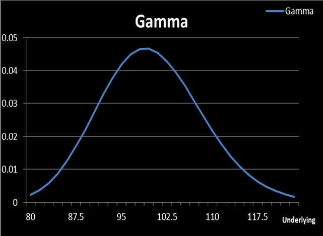
(Figure 5. Source: HyperVolatility Option Tool — Box)
We can see that Gamma is also changing along with the underlying. As the underlying comes closer to $91, Gamma increases to 0.01531 (it was 0.00374 when the underlying was at $90) which means that, at this point, the trader would need $107 (6,954*0.01531) Gamma and not $26 to offset her Gamma risk. Hence, she would have to buy more options. In other words, Gamma–hedging needs to be rebalanced as much as delta — hedging.
Delta–Gamma Hedging cannot offer full protection to the option position, but it can be deemed as a correction of the Delta–hedging error because it can reduce the size of each re–hedge and thus minimize costs.
From section 2.3 and 2.4, we can conclude that if Gamma is very small, we can solely use Delta hedging, or else we could adopt Delta–Gamma hedging. However, we should bear in mind that Delta–Gamma hedging is good only when Speed is small. Speed is the curvature of Gamma in terms of underlying price, which is shown in Figure — 6:
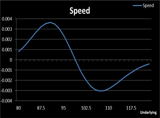
(Figure 6. Source: HyperVolatility Option Tool — Box)
Using the basic knowledge of Calculus or Taylor’s Series Expansion, we can prove that:
Δ Option Value ≈ Delta * ΔS + ½ Gamma * ΔS + 1/6 Speed * ΔS
We can see that Delta hedging is good if Gamma and Speed are negligible while Delta–Gamma hedging is better when Speed is small enough. If any of the last two terms is significant, we should seek to find other hedging methods.
2.5 Hedging Based on Underlying Price Changes / Regular Time Intervals
To avoid infinite hedging costs, a trader can rebalance her Delta after the underlying price has moved by a certain amount. This method is based on the knowledge that the Delta risk in an option position is due to the underlying movements.
Another alternative to avoid over–frequent Delta hedging is to hedge at regular time intervals, where hedging frequency is reduced to a fixed level. This approach is sometimes employed by large financial institutions that may have option positions in several hundred underlying assets.
However, both the suitable ‘underlying price changes’ and ‘regular time intervals’ are relatively arbitrary. We know that choosing good values for these two parameters is important but so far we have not found any good method to find them.
2.6 Hedging by a Delta Band
There exist more advanced strategies involving hedging strategies based on Delta bands. They are effective for finding the best trade–off between risks and costs. Among those strategies, the Zakamouline band is the most feasible one. The Zakamouline band hedging rule is quite simple: when the Delta of our position moves outside of the band, we need to re–hedge and just pull it back to the edge of the band. However, the theory behind it and the derivation of it are not simple. We are going to address these issues in the next research report.
Figure-7 provides an example of the Zakamouline bands for hedging a short position consisting of 1,000 European call options priced with S=$90, X=$110, T=30 days, r=0.5%, b=0, σ=30%:
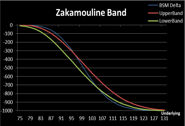
(Figure 7. Source: HyperVolatility Option Tool — Box)
In the next report, we will see how the Zakamouline band is derived, how to implement it, and will also see the comparison of Zakamouline band to other Delta bands in a quantitative manner.
If you found this research interesting, please have a look at the following ones too:
“Options Greeks: Delta, Gamma, Vega, Theta, Rho”
“Options Greeks: Vanna, Charm, Vomma, DvegaDtime”
“Extracting Implied Volatility: Newton-Raphson, Secant and Bisection Approaches”
“The Pricing of Commodity Options”
Visit HyperVolatility for more quant researches
This is information — not financial advice or recommendation. The content and materials featured or linked to are for your information and education only and are not attended to address your particular personal requirements. The information does not constitute financial advice or recommendation and should not be considered as such.

