Simple Image classification using deep learning — deep learning series 2

Published in

Intro to Artificial Intelligence

10 min readMay 4, 2018

Source : MathWorks (https://goo.gl/zondfq)

1. Introduction

We are going to discuss image classification using deep learning in this article. If we would like to get brief introduction on deep learning, please visit my previous article in the series. This article is going to discuss image classification using a deep learning model called Convolutional Neural Network(CNN). Before we get into the CNN code, I would like to spend time in explaining the architecture of the CNN. This project is done as part of the udacity deep learning course. It’s a great course and I encourage you to join the course.

2. Architecture

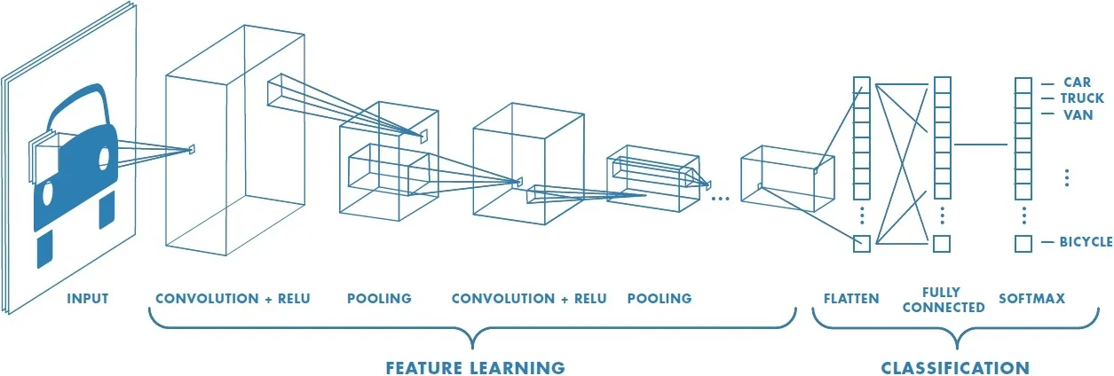
The Regular Neural Netowrks(NN) is not capable of dealing with images. Just imagine each pixel is connected to one neuron and there will thousands of neurons which will be computationally expensive. CNN handles images in different ways, but still it follows the general concept of NN.

Source: http://cs231n.github.io/convolutional-networks

They are made up of neurons that have learnable weights and biases. Each neuron accepts the inputs, action a dot product operation and follows the non-linearity function. And they still have a loss function (e.g. SVM/Softmax) on the fully-connected layer and all the tips & tricks we developed for learning regular NN still apply.

CNN is used as the default model for anything to deal with images. Nowadays there are papers that has mentioned about the use of Recurrent Neural Network(RNN) for the image recognition. Traditionally RNNs are being used for text and speech recognition.

Use of CNN helps to reduce the number of parameter required for images over the regular NN. Also, It helps to do the parameter sharing so that it can possess translation invariance.

Consider an example of a cat in an image. When we are trying to classify a picture of a cat, we don’t care where in the image a cat is. If it’s in the top left or the bottom right, it’s still a cat in our eyes. This is called translation invariance.

Convolution

Let’s dive into how convolution layer works. Convolution has got set learn-able filters which will be a matrix(width, height, and depth). We consider an image as a matrix and filter will be sliding through the image matrix as shown below to get the convoluted image which is the filtered image of the actual image.

Depend upon the task, more than one filter is available in the model to cater the different features. Feature might be looking for a cat, looking for colour etc. Filter matrix value is learned during the training phase of the model.

Padding is the another important factor in convolution. If you apply filter on the input image, we will be getting output matrix with less size than the original image. Padding comes into play, if we need to get the same size to output as input size.

Source: https://adeshpande3.github.io/A-Beginner%27s-Guide-To-Understanding-Convolutional-Neural-Networks-Part-2

Let’s consider the above example. Apply a zero padding of size 2 to that layer. Zero padding pads the input volume with zeros around the border. If we think about a zero padding of two, then this would result in a 36 x 36 x 3 input volume of 32 x 32 x 3.

Activation function

Activation functions are functions that decide, given the inputs into the node, what should be the node’s output? Because it’s the activation function that decides the actual output, we often refer to the outputs of a layer as its “activations”. One of the popular activation function in cnn is ReLu.

References:

https://en.wikipedia.org/wiki/Rectifier_(neural_networks)

Max pooling

Another important concept of CNNs is pooling, which is a form of non-linear down-sampling. There are several non linear functions that can do pooling, in which, max pooling is the most common one.

According to wikipedia, It partitions the input image into a set of non-overlapping rectangles and, for each such sub-region, outputs the maximum. The intuition is that the exact location of a feature is less important than its rough location relative to other features.

The pooling layer helps to reduce the spatial size of the representation, to reduce the number of parameters and amount of computation in the network. This also controls the over-fitting.

Fully connected

Finally, after several convolutional and max pooling layers, the high-level reasoning in the neural network is done via fully connected layers. Neurons in a fully connected layer have connections to all activations in the previous layer, as seen in regular neural networks. Their activations can hence be computed with a matrix multiplication followed by a bias offset.(Wikipedia)

Softmax

Softmax function calculates the probabilities distribution of the event over ’n’ different events. In general way of saying, this function will calculate the probabilities of each target class over all possible target classes. Later the calculated probabilities will be helpful for determining the target class for the given inputs.

Mathematically the softmax function is shown below, where z is a vector of the inputs to the output layer (if you have 10 output units, then there are 10 elements in z). And again, j indexes the output units.

3. Simple Image classification

I will explain through the code base of the project I have done through the Udacity deep learning course.

Our task is to classify the images based on CIFAR-10 dataset. The dataset consists of airplanes, dogs, cats, and other objects. Our aim is to build the CNN model, train them using the dataset, and classify the input images.

Download dataset

First of all get the dataset from CIFAR either through the script or direct download.

The dataset is broken into batches to prevent your machine from running out of memory. The CIFAR-10 dataset consists of 5 batches, named data_batch_1, data_batch_2, etc.

Pre-process functions

Normalization

The data is projected in to a predefined range (i.e. usually [0, 1]or [-1, 1]). This is useful when you have data from different formats (or datasets) and you want to normalize all of them so you can apply the same algorithms over them.

def normalize(x):
    """
    Normalize a list of sample image data in the range of 0 to 1
    : x: List of image data.  The image shape is (32, 32, 3)
    : return: Numpy array of normalize data
    """
    # TODO: Implement Function
    #Normalization equation
    #zi=xi−min(x)/max(x)−min(x)
    normalized = (x-np.min(x))/(np.max(x)-np.min(x))
    return normalized

One-hot encode

The input, x, are a list of labels. Implement the function to return the list of labels as One-Hot encoded Numpy array. The possible values for labels are 0 to 9. The one-hot encoding function should return the same encoding for each value between each call to one_hot_encode.

def one_hot_encode(x):
    """
    One hot encode a list of sample labels. Return a one-hot encoded vector for each label.
    : x: List of sample Labels
    : return: Numpy array of one-hot encoded labels
    """
    # TODO: Implement Function
    return np.eye(10)[x]

You can do preprocessing in two ways. One is when model is running and another one is preprocess all the data earlier. For saving the memory, it’s a good practice to preprocess the dataset earlier.

In this example, we preprocess the dataset using above functions earlier.

Build the network

In this section we build the model based on Tensorflow library.

Input

here we define the input variables in tensorflow.

import tensorflow as tfdef neural_net_image_input(image_shape):
    """
    Return a Tensor for a bach of image input
    : image_shape: Shape of the images
    : return: Tensor for image input.
    """
    # TODO: Implement Function
    return tf.placeholder(tf.float32, shape=(None, *image_shape), name='x')
def neural_net_label_input(n_classes):
    """
    Return a Tensor for a batch of label input
    : n_classes: Number of classes
    : return: Tensor for label input.
    """
    # TODO: Implement Function
    return tf.placeholder(tf.float32, shape=(None, n_classes), name='y')
def neural_net_keep_prob_input():
    """
    Return a Tensor for keep probability
    : return: Tensor for keep probability.
    """
    # TODO: Implement Function
    return tf.placeholder(tf.float32, name='keep_prob')

Convolution and Max Pooling Layer

This section defines the convolution and max pooling layer. Here is pseudo code for the layers:

1. Create the weight and bias using conv_ksize, conv_num_outputs and the shape of x_tensor.
2. Apply a convolution to x_tensor using weight and conv_strides.
3. Padding
4. Add bias
5. Add a nonlinear activation to the convolution.
6. Apply Max Pooling using pool_ksize and pool_strides.

def conv2d_maxpool(x_tensor, conv_num_outputs, conv_ksize, conv_strides, pool_ksize, pool_strides):
    """
    Apply convolution then max pooling to x_tensor
    :param x_tensor: TensorFlow Tensor
    :param conv_num_outputs: Number of outputs for the convolutional layer
    :param conv_ksize: kernal size 2-D Tuple for the convolutional layer
    :param conv_strides: Stride 2-D Tuple for convolution
    :param pool_ksize: kernal size 2-D Tuple for pool
    :param pool_strides: Stride 2-D Tuple for pool
    : return: A tensor that represents convolution and max pooling of x_tensor
    """
    
    
    #Define weight
    weight_shape = [*conv_ksize, int(x_tensor.shape[3]), conv_num_outputs]
    w = tf.Variable(tf.random_normal(weight_shape, stddev=0.1))
    
    #Define bias
    b = tf.Variable(tf.zeros(conv_num_outputs))
    
    #Apply convolution
    x = tf.nn.conv2d(x_tensor, w, strides=[1, *conv_strides, 1], padding='SAME')
    
    #Apply bias
    x = tf.nn.bias_add(x, b)
    
    #Apply RELU
    x = tf.nn.relu(x)
    
    #Apply Max pool
    x = tf.nn.max_pool(x, [1, *pool_ksize, 1], [1, *pool_strides, 1], padding='SAME')
    return x

Flatten Layer

Implement the flatten function to change the dimension of x_tensor from a 4-D tensor to a 2-D tensor. The output should be the shape (Batch Size, Flattened Image Size). This is one of the component of CNN architecture and we didn’t explain it in the above section.

def flatten(x_tensor):
    """
    Flatten x_tensor to (Batch Size, Flattened Image Size)
    : x_tensor: A tensor of size (Batch Size, ...), where ... are the image dimensions.
    : return: A tensor of size (Batch Size, Flattened Image Size).
    """
    # TODO: Implement Function
    batch_size, *fltn_img_size = x_tensor.get_shape().as_list()
    img_size = fltn_img_size[0] * fltn_img_size[1] * fltn_img_size[2]
    tensor = tf.reshape(x_tensor, [-1, img_size])
    return tensor

Fully-Connected Layer

def fully_conn(x_tensor, num_outputs):
    """
    Apply a fully connected layer to x_tensor using weight and bias
    : x_tensor: A 2-D tensor where the first dimension is batch size.
    : num_outputs: The number of output that the new tensor should be.
    : return: A 2-D tensor where the second dimension is num_outputs.
    """
    # TODO: Implement Function
    #weights
    w_shape = (int(x_tensor.get_shape().as_list()[1]), num_outputs)
    weights = tf.Variable(tf.random_normal(w_shape, stddev=0.1))
    
    #bias
    bias = tf.Variable(tf.zeros(num_outputs))
    x = tf.add(tf.matmul(x_tensor, weights), bias)
    output = tf.nn.relu(x)
    return output

Full model

This function call all the individual section mentioned above to make a full model. The function takes in a batch of images, x, and outputs logits. Use the layers you created above to create this model. We use drop_out(regularisation) for avoiding the overfitting.

def conv_net(x, keep_prob):
    """
    Create a convolutional neural network model
    : x: Placeholder tensor that holds image data.
    : keep_prob: Placeholder tensor that hold dropout keep probability.
    : return: Tensor that represents logits
    """
    # TODO: Apply 1, 2, or 3 Convolution and Max Pool layers
    x = conv2d_maxpool(x, 32, (3, 3), (1, 1), (2, 2), (2, 2))
    x = conv2d_maxpool(x, 32, (3, 3), (2, 2), (2, 2), (2, 2))
    x = conv2d_maxpool(x, 64, (3, 3), (1, 1), (2, 2), (2, 2))
        # TODO: Apply a Flatten Layer
    # Function Definition from Above:
    x = flatten(x)
        # TODO: Apply 1, 2, or 3 Fully Connected Layers
    #    Play around with different number of outputs
    # Function Definition from Above:
    #   fully_conn(x_tensor, num_outputs)
    x = fully_conn(x, 128)
    x = tf.nn.dropout(x, keep_prob)
    
    
    # TODO: Apply an Output Layer
    #    Set this to the number of classes
    # Function Definition from Above:
    #   output(x_tensor, num_outputs)
    result = output(x, 10)
    
    
    # TODO: return output
    return result
"""
DON'T MODIFY ANYTHING IN THIS CELL THAT IS BELOW THIS LINE
"""##############################
## Build the Neural Network ##
############################### Remove previous weights, bias, inputs, etc..
tf.reset_default_graph()# Inputs
x = neural_net_image_input((32, 32, 3))
y = neural_net_label_input(10)
keep_prob = neural_net_keep_prob_input()# Model
logits = conv_net(x, keep_prob)# Name logits Tensor, so that is can be loaded from disk after training
logits = tf.identity(logits, name='logits')# Loss and Optimizer
cost = tf.reduce_mean(tf.nn.softmax_cross_entropy_with_logits(logits=logits, labels=y))
optimizer = tf.train.AdamOptimizer().minimize(cost)# Accuracy
correct_pred = tf.equal(tf.argmax(logits, 1), tf.argmax(y, 1))
accuracy = tf.reduce_mean(tf.cast(correct_pred, tf.float32), name='accuracy')

In the above code, we are using loss and optimiser which is not explained above. Both of them required for the CNN to do the training. Loss determine the loss function of the forward pass on each run and optimiser does the backpropogation for the learning purpose based on the loss function.

Training

Training can be done by using tensorflow’s session variable.

def train_neural_network(session, optimizer, keep_probability, feature_batch, label_batch):
    """
    Optimize the session on a batch of images and labels
    : session: Current TensorFlow session
    : optimizer: TensorFlow optimizer function
    : keep_probability: keep probability
    : feature_batch: Batch of Numpy image data
    : label_batch: Batch of Numpy label data
    """
    # TODO: Implement Function
    session.run(optimizer, feed_dict={
        x: feature_batch,
        y: label_batch,
        keep_prob: keep_probability
    })