Brain MRI Segmentation using Deep Learning

Published in

Kuzok

6 min readSep 16, 2019

This project was a runner-up in Smart India Hackathon 2019. The problem statement was Brain Image Segmentation using Machine Learning given by Department of Atomic Energy, Government of India, in the complex problem statements category.

You can find complete project here.

The method segments 3D brain MR images into different tissues using fully convolutional network (FCN) and transfer learning.

A Fully Convolutional neural network (FCN) is a normal CNN, where the last fully connected layer is substituted by another convolution layer with a large “receptive field”. The idea is to capture the global context of the scene (Tell us what we have in the image and also give some very rough idea of the locations of things).

Transfer learning make use of the knowledge gained while solving one problem and applying it to a different but related problem. For example, knowledge gained while learning to recognize cars can be used to some extent to recognize trucks.

As compared to existing deep learning-based approaches that rely either on 2D patches or on fully 3D FCN, this method is way much faster: it only takes a few seconds, and only a single modality (T1 or T2) is required. In order to take the 3D information into account, all 3 successive 2D slices are stacked to form a set of 2D “color” images, which serve as input for the FCN pre-trained on ImageNet (a popular image database) for natural image classification.

Modalities T1 and T2 are radiology terms depending on types of tissues. In the dataset, we have both T1 weighted images and T2 weighted images, and we will use just single modality images to predict the results.

Preprocessing:

In order to take the 3D information into account, all 3 successive 2D slices are stacked to form a set of 2D color images, which serve as input for the FCN pre-trained on ImageNet for natural image classification.

Histogram equalization (only for T1 modality)
Stack 3 continue slices as a RGB image
Flip and rotate for [$0,\pm 5,\pm 10,\pm 15$] for data augmentation
Crop to reduce background in image and ensure width and height can be divided by 16

Network Architecture:

Before jumping in the network architecture, lets first understand VGG16:

VGG16:

VGG16 is a convolutional neural network model built using Convolutions layers (used only 3*3 size ), Max pooling layers (used only 2*2 size), and Fully connected layers at end having a total of 16 layers.

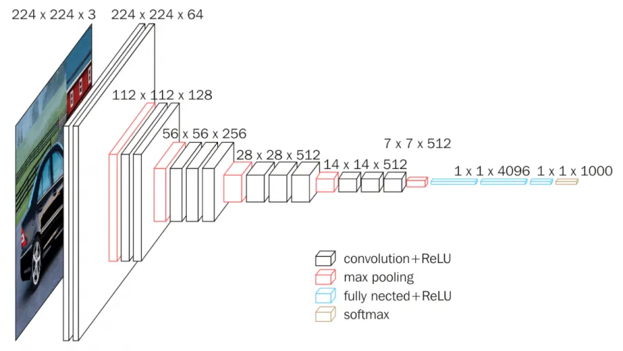
The input to cov1 layer is of fixed size 224 x 224 RGB image. The image is passed through a stack of convolutional (conv.) layers, where the filters were used with a very small receptive field: 3×3 (which is the smallest size to capture the notion of left/right, up/down, center). In one of the configurations, it also utilizes 1×1 convolution filters, which can be seen as a linear transformation of the input channels (followed by non-linearity). The convolution stride is fixed to 1 pixel; the spatial padding of conv. layer input is such that the spatial resolution is preserved after convolution, i.e. the padding is 1-pixel for 3×3 conv. layers. Spatial pooling is carried out by five max-pooling layers, which follow some of the conv. layers (not all the conv. layers are followed by max-pooling). Max-pooling is performed over a 2×2 pixel window, with stride 2.

Three Fully-Connected (FC) layers follow a stack of convolutional layers (which has a different depth in different architectures): the first two have 4096 channels each, the third performs 1000-way ILSVRC classification and thus contains 1000 channels (one for each class). The final layer is the soft-max layer. The configuration of the fully connected layers is the same in all networks.

All hidden layers are equipped with the rectification (ReLU) non-linearity. It is also noted that none of the networks (except for one) contain Local Response Normalisation (LRN), such normalization does not improve the performance on the ILSVRC dataset, but leads to increased memory consumption and computation time.

Our model:

We rely on the 16 layers VGG network pre-trained on millions of natural images in ImageNet for image classification. For our application, we discard the fully connected layers at the end of VGG network, and keep the 5 stages of convolutional parts called “base network”. This base network is mainly composed of convolutional layers, Rectified Linear Unit (ReLU) layers for non linear activation function, and max pooling layers between two successive stages.

We discard the red-part(fully connected layers) of VGG16

The four max pooling layers divide the base network into five stages of fine to coarse feature maps. We add specialized convolutional layers (with a 3 × 3 kernel size) with K (e.g. K = 16) feature maps after the convolutional layers at the end of each stage. We resize all the specialized layers to the original image size, and concatenate them together. A last convolutional layer with kernel size 1 × 1 is appended at the end that combines linearly the fine to coarse feature maps in the concatenated specialized layers, to produce the final segmentation result.

Simply put, we stack successive 2D slices of a 3D volume to form a set of 2D “color” images, these 2D images constitute the input of a FCN based on VGG network, pre-trained on the ImageNet dataset. We discard the fully connected layers, and we add specialized convolutional layers at the end of each of the five convolutional stages in VGG network. A linear combination of these specialized layers (i.e. fine to coarse feature maps) results in the final segmentation.

Why our model?

Since we are using transfer learning, a novel approach in this field, so we do not need to train our model from scratch which makes it very fast in training in comparison to other models.
Stacking 3 successive 2D slices allows us to make a RGB image, another novel idea.This representation enables us to incorporate some 3D information, while avoiding the expensive computational and memory requirements of fully 3D FCN.
Using Transfer Learning we do not need many training images, so we could train our model very well only on a few training images.
We are also using traditional data augmentation methods like rotating, cropping and flipping the images in training set for improving our model.

Results:

We used BraTS 2018 dataset. The dataset contains .nii files, which are basically 3d images having layers of stacked 2d images. We are using Papaya viewer integrated into django app for input and showing prediction. The app takes the input as zip file, unzips and runs the model on it and shows the prediction.

Giving input and prediction: