Part 5 : Row Picture and Column Picture

There are two ways to represent system of linear equations as matrices.

Row Picture

In row picture representation we make a coefficient matrix, a variable matrix and a constant matrix. We have discussed this earlier. It is advisable to open Part 1 in a another tab because we have to reference it a lot of times in this article.

Assuming a system of linear equations as follow :

3x-5y = 6 →(1)

x+y = 4 →(2)

3x+y = 0 →(3)

Representation of this system in row picture would be :

After multiplying these matrices we will get our equations back

Row picture on graph

The row picture of (1), (2) and (3) could be plotted on graph as :

We can see from the graph that this system does not have one unique solution

To find solution of system of linear equations from Row picture, we look at graph and see if there is any one point of intersection for all the lines, that point is called solution for the system of equations.

If there is no common point, then there is no solution for the system of equations (as seen in the case above).

Column Picture

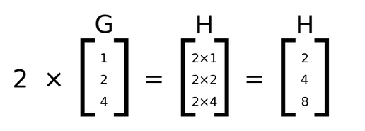
A column picture is where coefficient matrix if formed separately for each variable. After that variables are multiplied with their coefficient matrices (scalar multiplication) and added together.

Then, it is equated to constant matrix.

Taking the system of linear equations (1), (2) and (3), the column picture would be as follows :

“x” and “y” are scalars being multiplied with their corresponding coefficient matrices

Column picture on graph

To show column picture on graph, we treat individual coefficient matrices as vectors and plot those vectors on graph.

Blue vector is coefficient matrix of X ,Red vector is coefficient matrix of Y and Green Vector is Constant matrix

To find solution of system of equations from Column picture we multiply coefficient matrices with different values of variables (x and y ) and add them together (vector addition is similar to matrix addition). If the result comes to be equal to the constant matrix then those values of x and y are called solution of system of linear equations.

For this example, as we have seen in row picture there is no solution. Hence, for no value of x and y in column picture the sum vector is going to be equal to constant matrix (or vector).

While finding solution for any system of linear equations we can encounter one of the three cases

One Unique solution

Consider a system of linear equation :

4x+y = 9→(4)

2x-y = 3→(5)

5x-3y = 7→(6)

Plotting these equations as row picture and column picture on graph :

Row Picture of (4), (5) and (6)

Column Picture of (4), (5) and (6)

To verify solution x= 2 and y=1, from column picture we substitute their values and calculate.

So, the result is equal to constant matrix. Hence, x=2 and y=1 is one unique solution of system of equations (4), (5) and (6).

Infinitely Many Solutions

Consider a system of linear equations :

x+2y = 4→(7)

2x+4y = 8→(8)

Plotting these equations as row picture and column picture on graph :

Both lines overlap each other

Here, we have solutions but they are infinitely large in number (because both lines intersect at almost every point).

Seems like red vector and green vector are scalar multiplication products of blue vector

So, there could be infinitely large number of values for x and y such that column picture returns constant matrix.

No Solution

Consider a system of linear equation :

x+y = 4→(9)

x+y = 8→(10)

x-y = 0→(11)

Plotting these equations as row picture and column picture on graph :

There is no point of intersection for all three lines

We can see that there is no possible values of “x” and “y”

Multiplication through row and column picture

Other than the way of matrix multiplication discussed earlier, we can do multiplication in two more ways

Row Picture multiplication

When individual columns of one matrix is multiplied with rows (scalar multiplication) of another matrix and resulting matrices are added together.

Assuming that we have to multiply these two matrices

Column 1 of first matrix (4) is multiplied with Row 1 of second matrix, Column 2 of first matrix (5) is multiplied with Row 2 of second matrix and so on

Result is exactly what we would have expected from normal multiplication method

Column Picture multiplication

When individual rows of one matrix is multiplied with columns (scalar multiplication) of another matrix and resulting matrices are added together.

Assuming these are the two matrices we want to multiply

Row 1 of second matrix (3) is multiplied with Column 1 of first matrix, Row 2 of second matrix (4) is multiplied with Column 2 of first matrix and so on

Result is same as what we would have got with normal multiplication method

Read Part 6 : Gaussian Elimination

You can view the complete series here
I’m now publishing at avni.sh

Connect with me on LinkedIn.