Convolutional Neural Networks For All | Part II
The mentor-curated study guide to summarize all lectures from the Coursera Deep Learning Specialization course 4
If you’re not a Deep Learning expert, chances are that the Coursera Convolutional Neural Networks course kicked your behind. So much information, so many complex theories covered in such a short time! Countless times pausing the lectures, rereading additional material and discussing topics later led us, a group of official mentors, to decide a learner study guide is worth the effort.

Part I reviews the broad concepts covered in this course. Part II summarizes every single lecture for you. Part III will offer a deeplearning.ai dictionary to help you sort through the jungle of acronyms, technical terms and occasional jokes from grandmaster Ng once we’ve finished course 5.
Let’s dive deeper into the bewilderment of interesting information by recapping every lecture.
Week 1
Computer Vision — CV allows computer programs to process images and videos to recognize the environment. It is heavily used in applications like face recognition or helping self-driving cars identify cars or pedestrians.

Edge Detection Example — Convolutional Neural Networks (CNNs) are at the heart of most CV applications. CNNs use the convolution operation to transform input images into outputs. A single step of convolution multiplies and sums the pixel values of an image with the values of a filter. This filter can be of shape 3x3. Next, the filter is shifted to a different position and the convolutional step is repeated until all Pixels were processed at least once. The resulting matrix eventually detects edges or transitions between dark and light colors and eventually more complex forms. The more filters you apply, the more details the CNN is capable to recognize.

More Edge Detection — Horizontal edge detection works by creating a horizontal edge in the filter and vice versa for vertical edges. The weights for edge filter detection can be learned through backpropagation instead of manually coding the values because images generally have many complex edges.
Padding — Add an additional pixel border around the image to preserve the original image size. This helps to prevent shrinking the input through convolutional filtering. “Valid” padding means that you use zero padding and the size of the image shrinks. “Same” padding adds as much padding as is needed to keep the dimension of the output equal to the input.

Strided Convolutions — You can move the convolutional frame by more than one “stride”, meaning you skip as many pixels as strides.
Convolution over volumes — When filtering a three-layered (RGB) image, you can also create a three-layered filter. You can still use multiple filters and stack the results like before.

One layer of a convolutional network — A convolution network is very similar to a vanilla neural network. Basically, you adjust the input with the weights and a bias term: w * a + b. This is the result of a filter convolution. You calculate the input and output based on the previous layer.
A simple convolution network example — Stack multiple convolution results behind each other to create a final layer. Generate the result through logistic or softmax output and use backpropagation to minimize the loss function.
Pooling layers — Max pooling selects the maximum value of all selected squares to make feature detection more robust. Average pooling simply uses the average of all values, but max pooling is generally preferred. Neither pooling method requires parameters and so backpropagation also doesn’t need to learn any parameters. 👍

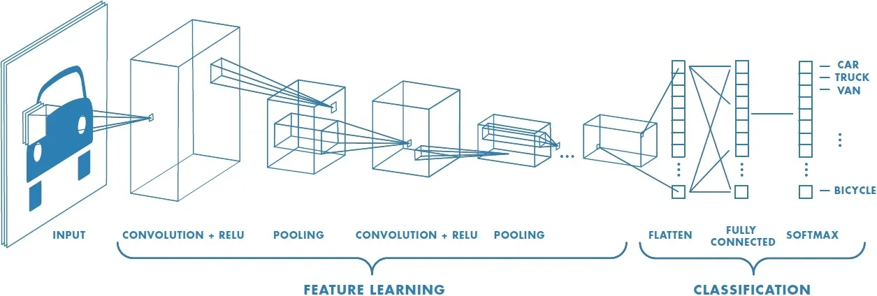
Convolutional neural network example — CNN consists of a convolutional layer followed by a pooling layer. At the end, you can use general fully connected layers, which are just flattened pooling layers and eventually generate a result.
Why Convolutions? — The main advantages of using convolutions are parameter sharing and sparsity of connections. Parameter sharing is helpful because reduces the number of weight parameters is one layer without losing accuracy. Additionally, the convolution operation breaks down the input features into a smaller feature space, so that each output value depends on a small number of inputs and can be quickly adjusted.
Week 2
Why case studies? — Just like reading other people’s code teaches you how to code, observing other peoples network architectures gives you an intuition which network structure might work for your problem.
Classic networks — This lecture explains the network architectures LeNet-5, AlexNet, and VGG. LeNet-5 used a conv-avgpool-conv-avgpool-fc-fc structure, shrinking the size of the image while increasing the filter dimensions. AlexNet is longer and much larger in terms of parameters. VGG really simplifies the architecture because it always uses a 3x3 filter and max pool with stride 2x2 and eventually becomes the largest network.


Residual networks — They allow you to train very deep networks. An input skips multiple layers up to a point much deeper in the network. This method is very effective at training deep neural networks.
Why do ResNets work? — ResNets improve the performance on the training set, which is a prerequisite to do well on the validation and test sets. It is easy for a residual block to learn the identity function by adding skipped connections.
Networks in networks and 1x1 convolutions — A 1x1 convolution multiplies every element of a convolutional block with a 1x1xC filter to output a scalar. This shrinks the number of filters when they become too large. Simply convolve a block with a 1x1 filter with the desired amount of filters. Use pooling at the next step to shrink the height and width of the input.
Inception network motivation — An inception network allows you to apply multiple filters and pooling layers to the network. It stacks multiple convolution outcomes together. The large computational cost is prevented by shrinking the input with 1x1 filters first and then generating the output block.

Inception network — Is a large concatenation of inception modules, also known as GoogLeNet.

Using open-source implementations — Make it a habit to look for open-source implementations first before you implement a network from scratch. Many researchers and practitioners regularly open-source their work. Feel free to give your two cents back to the community by open-sourcing your own work as well. 🤓
Transfer learning — Use the weights and architectures from a pre-trained neural network to get started with your deep learning task. Freeze the earlier layers of an existing model (use the existing architecture and their weights). Next, cut off the last softmax layer and replace it with your own layer to adjust the predictions to your use case. Feel free to reference this great blog post by Sebastian Ruder for additional explanations.


Data augmentation — In many cases, the key to computer vision is to get more data, so many techniques are used to augment existing data. Mirroring is one technique, simply flipping an image on the vertical axis. Random cropping is used to crop random parts of an image. Rotation or shearing as a form of image distortion can also be used. Color shifting is used to add integers to the RGB channels of pictures. Use one CPU thread to load the data and implement distortions during training.
State of computer vision — If you have a lot of data, simple algorithms might perform fine and you don’t need a lot of hand-engineering. If you don’t have enough data, try hand-engineering, adjusting the network architecture or transfer learning. Deep learning has two sources of knowledge, labeled data, and hand-engineering/network architecture. Depending on your situations, you can aim to improve either source.
Week 3
Object localization — In order to classify objects, you need to localize them first. This lecture covers three methods of classification: Image classification, Classification with localization and Landmark Detection. Image classification classifies an image, e.g. contains a cat or not. Classification with localization classifies an object with its bounding box in an image. Detection is used to locate multiple objects in an image. The output of the CNN has the following format as shown in the image below. The CNN object detection minimizes the loss function, e.g. the squared error, between y and predicted y.


Landmark detection — Is used to define landmarks in an image. Can be used to mark eyes in a face. Then train the CNN to output the locations of these landmarks. The identities of the landmarks have to be consistent in the entire training set, meaning the first landmark always has to mark the corner of the left eye, for example. It can also be used to detect the whole shape of a face or the action that an athlete performs in an image.
Object detection — Detect objects in an image through “sliding windows”. First, train a CNN on closely cropped pictures of the object. Next, create a window frame of a smaller size than the image and place it in a corner over the image. Run a CNN to determine if this window frame matches the cropped version of the object. Move the window to the next part of the image and detect the object again. Repeat this procedure for the entire image. Object detection is very computing intense and is prone to miss the object if the sizes of the window and the object don’t match.

Convolutional implementation of sliding window — A convolutional implementation of the “sliding windows” method is much more efficient. Run a CNN over the entire image once. The final convolutional layer shows the object detection for every sliding windows frame in one iteration.
Bounding Box Prediction — The YOLO algorithm helps you detect accurate bounding boxes for object detection. To train a CNN using YOLO, you first have to place a grid over your training image, often a 19x19 grid is used. Next, you create the output labels for every grid. Does this grid contain the center of a relevant object? If so, draw a bounding box around it and label the output vector y accordingly. This way, label as many images as possible. Your CNN architecture has to result in the final layer having the shape of the grid cells for width and height and as many channels as the number of elements in a single y vector. If you want to detect five classes of objects, your output vector y has 10 elements. 1 element to indicate whether an object exists or not, 4 elements to indicate the objects center and its width and height plus 5 elements, indicating the class the object belongs to. Backpropagation now adjusts the weights of the CNN so that it learns to identify the objects. You only need a single forward propagation step to identify the objects in an image.
YOLO algorithm — The algorithm, short for “You Only Look Once”, is more accurate compared to “sliding windows”. It returns the exact boundaries of the object even if the window size doesn’t exactly match the object.


Intersection over union — Is used in non-max suppression to support YOLO finding the exact boundaries of the object. The formula divides the size of the object by the size of the union of two windows. If IoU > 0.5, then the intersection contains the object. IoU is a measure of the overlap of two bounding boxes.


Non-max suppression — It cleans up the result of the YOLO detections in an image. YOLO sometimes identifies the same object in multiple grid cells with slightly different bounding boxes. Use non-max suppression to find the true bounding box of the object with the help of IoU. All boxes with a high IoU will be suppressed. First, discard all boxes with a probability of containing the object < 0.5. Next, output the box with the highest probability and suppress all boxes with an IoU > 0.5.
Anchor boxes — Allows CNN to detect two overlapping objects, e.g. dog standing in front of a bike. It is used to learn shapes of wide cars and tall pedestrians in images. First, create anchor box shapes. If center points of two objects overlap, associate them with two different anchor boxes. The object is now assigned to the grid cell with contains the object center point and to the anchor box which has the highest IoU with grid cell. The output y is stacked together with top part belonging to anchor box 1 and second part to anchor box 2. If only an object from anchor box 2 is in this grid cell, y will only fill in values for lower part of output y and “don’t care” values for the upper part, corresponding to anchor 1.
Putting it together — YOLO algorithm: 2 anchor boxes are used to detect multiple objects in an image. The output layer will be of the following shape: 3x3 (grid cell shape) x2 (# of anchor boxes) x8 (output vector containing probability of image detection, 4 numbers to describe location in object, and 3 numbers to describe the class that is detected). First, the CNN generates two anchor boxes for every grid. Second, the anchor boxes with a low probability are discarded. Third, non-max suppression is used to detect the final bounding boxes of the objects.

(Optional) Region Proposals — R-CNN classifiers detect interesting regions in an image and classify those rather than through using grids. A segmentation algorithm creates about 2k blobs and tries to detect interesting regions and objects out of these regions. For more information on the quite popular variations of R-CNNs, check out this great post or Facebook’s latest Detectron library.

Week 4
What is face recognition? — The lecture distinguishes between two sets of problems: face verification and face recognition. Verification is used to verify that the person of interest is truly who they claim to be and it is a 1:1 problem. Face recognition is the problem of recognizing if a face belongs to a face from a database of K humans and it is a 1:K problem. Face recognition is a very tough problem because if face verification is 99% accurate, then the larger the database of people, the larger the chance for an error. If your database has 10,000 people that you want to correctly identify, a face recognition error of 1% will yield 100 misclassified examples.

One-shot-learning — Refers to the need to recognize a person just given one example. The neural net learns a similarity function which is small when two pictures from the same person are given to the net and large if different persons are on those pictures, like in the collage below.

Siamese network — Is used to describe the difference between the last fully connected output layer of two images. Train the same CNN with two images and compare last output layer. Next, learn the parameters so that the difference is small between similar images of the same human and large between images of different humans.
Triplet loss — A method to train a CNN’s similarity function. Always use three images at the same time, an anchor image, a positive and a negative example of the human you want to recognize. Add a margin to prevent the function from only outputting zeros. Choose triplets that are hard to train, e.g. similar images from different persons. To improve performance, use multiple images of the same person in the training set.

Face verification and binary classification — Instead of using triplet loss, you could also use the convolutional results of two images and then compute a logit function at the end if persons are same or not to train a similarity function. Use a siamese network and use the last FC layer units to input them into a logistic unit, so that it becomes a binary classification.
What is neural style transfer? — Generate a new image which combines style and content from two other images. Often used to mix a real-world picture with the image of a painting.

What are DeepConvnets really learning? — Shallow layers of a CNN learn simple forms and deeper layers learn gradually more complex forms.

Cost function — Generate an image G with random pixel values. Next, define a cost function for the content C and style S images with regard to generated image G. Add both cost functions and add a bias term to define the cost function for the generated image J(G). Use gradient descent to minimize J(G) and update G, meaning you will update the pixel values so that G will look more like S and C.

Content cost function — Is used to check how similar the contents are of the generated image G and the content image C. Choose a layer in the middle of the CNN so that the content is abstract enough to be mixed with the style image. If you choose a later layer you will simply make sure that, e.g. a dog is somewhere in G because a dog is also in C. Pick a layer in CNN and run forward propagation for C and G until this layer. Compare the activations and optimize the cost function J(C). J(C) is the element-wise sum-of-squares difference between pixel values of C and G. This way, J(C) incentivizes G to become similar to C.

Style cost function — The core of the style cost function is measuring the correlation between the channels. Again, choose a hidden layer to measure the style of S. Style is the correlation between the activations across channels. How correlated are activations across channels? The correlation measure tells you how similar the outputs of the channels are. The correlation has to be similar to the generated image G so that G and S have the similar style. The key is to compute two “Gram” matrices which calculate every possible pair of filter activations across the channels.
You then take this Gram matrix from S and compare it to G. Next, you sum all of these target styles vs. the generated style differences and try to minimize the cost J(S).

The diagonal of this gram matrix learns the correlation between the channels and thus is adjusted. J(S) now aims to minimize the squared difference (Frobenius difference) between two gram matrices. Additionally, you get the best results from summing over multiple hidden layers, so that generated image has lower and higher level features from S. But the focus remains on the gram matrix.

1D and 3D generalizations — Convolutions can also be used to transform 1D or 3D inputs.
Disclaimer: All credit is due to deeplearning.ai. While I’m a mentor, I’m merely summarizing and rephrasing the content to help learners progress.
Part II is a wrap, review Part I here and continue to Part III. If you think this post was helpful, don’t forget to show your 💛 through 👏 👏 👏 and follow me to hear more articles about Deep Learning, Online Courses, Autonomous Cars, and Life. Also, check these posts about the Deep Learning Specialization. Please comment to share your opinion. Cheers! 🙇