Linear Regression (without any complex maths, yay!)
What does that thing written above mean?
Okay… hear me out!
The things you learned in school… aren’t useless!
That might have been a controversial thing to say as most students love calling schools out for teaching us “useless maths stuff” instead of “taxes and how to be a quadrillionaire in a week”. But it is pretty true.
As I am studying more and more about the field of Machine Learning, I’ve been thanking the things I learned in school for the first time in my whole life!
One such thing that school helped me in understanding was Linear Regression.
You might be thinking, “What? When did they teach Linear Regression in school?”. Which… is a pretty valid question. We weren’t taught “Linear Regression”, but the Equation for a straight line.

If you understand what y = mx + b means then you are halfway there in understanding what Linear Regression is.
Linear Regression is nothing else but fitting a straight line through a bunch of data in order to predict new values.
Yup! That’s it! That’s all there is to understanding what Linear Regression does. It is another one of those “fancy-sounding terms which are pretty simple in reality”.

Linear Regression comes under the umbrella of Regression algorithms and is the simplest one out of them all. But don’t underestimate it just because it’s basic.
Linear Regression comes in two flavors - Vanilla and Butterscotch.
I mean, Simple Linear Regression and Multiple Linear Regression.
Flavors of Linear Regression
As I said above, Linear Regression comes in two flavors, Simple Linear Regression and Multiple Linear Regression. Let’s lick both of these, one by one, and understand why they are different.
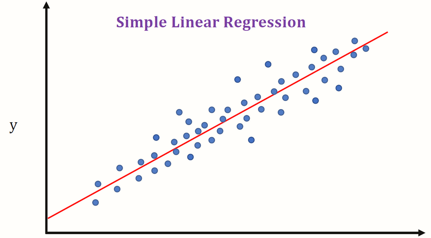
Simple Linear Regression
As the name suggests Simple Linear Regression is the simpler one out of the two flavors.
It is called “simple” because it only uses one variable to predict new outcomes.

The equation above is the equation for Simple Linear Regression. If you look closely it won’t feel much different from the equation in Image 1. The only change here is in the name of the variables.
c (intercept)has been changed to beta_0, and m (slope) has been changed to beta_1.
x1 here is the main variable that we’ll be using to predict y, and beta_1 is the slope of the line made by plotting x1 against y.
Multiple Linear Regression
As the name suggests this flavor uses multiple variables for predicting new values.

The equation above is the equation for Multiple Linear Regression. If you look closely it won’t feel much different from the equation in Image 3. The only change here is that there are a few more terms added to the equation.
x1, x2, x3, and so on are all the variables that we’ll be using to predict y, and beta_1, beta_2, beta_3, and so on are the slope of the line made by plotting those variables against y.
(Did he seriously just copy the description of Simple Linear Regression, made a few changes, and pasted them here?)
(Yes… he did!)
How to calculate the betas?
Now that you know the equations for both the flavors, you might be having the question “How do I calculate those betas?”.
Well, buckle up Buckaroo because we’ll be going on a whole rollercoaster ride for calculating those betas.
In this ride, you’ll be learning about methods like OLS (Ordinary Least Squares) and Gradient Descent.
(If you want to know what Gradient Descent is click here. This guy wrote a pretty cool article, so I would like him to get a few impressions…)
Sources -
- Image 1-https://cdn.kastatic.org/googleusercontent/ovqBFMBrGMZ1PfJ6XMADhigWzTDP5AaEmaEIAnNKjwiOlLuGd46fET8QeRqB9LZ9XVpvoX85lbz0YIYsV-98UTCs
- Image 2- https://miro.medium.com/max/1400/1*Cw5ZSYDkIFpmhBwr-hN84A.png
- Image 3- Made by the author using this website.
- Image 4- Made by the author using this website.