Overture puts you in the driver’s seat of its vision API
An intuitive guide to hyperparameter selection for image classification.

At Overture, we are building a computer vision platform with the belief that our users should have full control over their computer vision models. A rigid API just doesn’t cut it for the specialized applications that they are building. This is why we provide fully-customizable APIs:

In this article we will go over the hyperparameters of a convolutional neural network (CNN). This is the algorithm at the heart of Overture’s image classification tool. For those who do not know, hyperparameters are parameters that are set before the actual training begins. They control the training process of a model training algorithm. We will not go too deep into the technical details but will rather follow a practice approach on how these hyperparameters influence the training process. Spoiler alert, it’s often an iterative process to find the best set of hyperparameters. At the end of the article you can find a demo video on how you can do all of this in just a few clicks on our platform.
Data Augmentation

The first set of hyperparameters are related to augmenting the dataset. Most people are well aware of the fact that deep learning algorithms are super-hungry for data. This is one of the reasons why it’s common practice to augment your dataset with some simple image transformation techniques that are randomly applied on your images. But when do you use it and when do you use which technique? Well, it depends.
When do you (not) use data augmentation?
It’s contrary to what you might think, but data augmentation is not only useful for small datasets. Let’s assume you’re lucky and you have a lot of different images of the objects you want to recognize. I’m talking thousands or at least a few hundred per label. You could think you have a pretty defendable case for not using data augmentation. But even in this scenario, could it be worthwhile using data augmentation. The clue is that not only the number of images but also the dissimilarity between the images is important. E.g. if the model is trying to distinguish cats from dogs and all dogs are right-facing and all cats left-facing, it is possible that the model will figure that all left-facing animals are cats (even when they are dogs). By flipping random images left/right, this effect is mitigated.
There are some cases however in which data augmentation harms the performance of your model. Imagine you’re trying to distinguish some objects based on their orientation or color. E.g. when you’re trying to distinguish left from right shoes in images or green apples from red ones. In this case you would not perform left/right or color augmentation options respectively. The same is true for top/bottom flips. When you’re trying to distinguish objects based on their size, you do not perform the scaling augmentation. The same logic applies to shape-related classification and skew augmentation.
Last but not least, is (Gaussian) noise augmentation. This type of augmentation adds random noise pixels to the image and combats overfitting in this way. We will discuss overfitting further down in the paragraph about drop-out. Besides overfitting, it also makes the model more robust towards noise in the future.
Our general guideline for data augmentation: If the object still belongs to the same category when the augmentation is applied, the augmentation will likely add information that will help improve your model. Try it. It’s often the easiest and most powerful tool to improve your model.
You now have an idea on when (not) to use augmentation, but how many samples do you add? There is no fixed rule for this. It depends on how many original images you already have in your dataset and how diverse the images are. We recommend that at least 20% of your dataset exists of original images. You can however augment even more. But more data also means that training your model will take longer. If you want to know more about the effects of augmentation on your model, this article sets up a pretty nice experiment.
Hyperparameters related to training the network
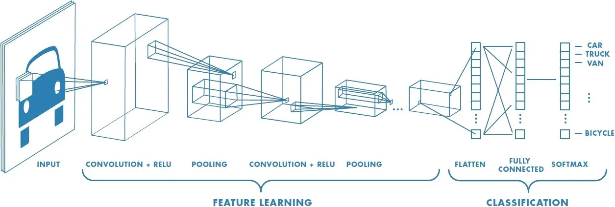
The next category of hyperparameters are related to the actual training process. To train our models at Overture, we use the power of transfer learning. This is a technique that leverages the learnings of a previously trained network. During the first step of transfer learning, we load this model that is already trained on millions of examples, we remove the last classification layers and add new ones (See Figure 1 for a visual representation of a CNN). We keep the feature learning layers of the network (convolutional base) and signal the network not to change their parameters. This technique is called “freezing the convolutional base”. The new classification layers are trained by feeding the network images of the new categories you want to recognize.
All of this makes a lot of sense intuitively. The convolutional base of the network already knows how to recognize basic image features (edges, colors, etc). We just use these output features (bottleneck features) to train the last classification layers for your new categories. In summary, you can consider the first part of the network as a collector of relevant information. The second part uses this information as input to learn to make the actual decision of what’s on the image.
After the training of the new classification layers, you can add Finetuning. This is optional. Let’s discuss both steps in more detail and the parameters that govern them.
Step 1: Classification layer training

Epochs and learning rate
To start the retraining of the new classification layers (green box on Figure 2), you need to specify how many training units or epochs the model can learn. Conversion usually occurs within 10 to 15 epochs with our algorithms and can be inspected in the output metrics graphs. We will tell you more about the metrics of a neural network in the next blogpost.
Per step you use a certain learning rate. This is the rate at which the network evolves to its optimal state. When this rate is too low, we need many epochs to reach the optimal state. When it is too high, we might overshoot the optimal state. A great visualization of the problem can be found in Figure 3.

The default learning rate is 0.003. This works good for most cases. But if you want to find the best learning rate for yourself, we recommend the following technique:
- you start with a high learning rate, like 0.1.
- You schedule a training job on the platform of maximum 5 epochs for retraining the classifier layers and check wether the loss improves. The loss is a measure for the inconsistency between what the network has learned and the actual data.
- When your learning rate is too high, the loss will not decrease after each epoch and the validation loss will be very high.
- When this is the case, you exponentially lower the value. So, you try the next learning rate 0.01 and perform this process iteratively if necessary, until the loss consistently decreases during the first few epochs. This will be the maximum learning rate you can use.
Practically, this approach seldom costs us more than 3 iterations, so it is usually in the range of [0.1,0.0001 ]. But if you want to find the optimal learning rate in a more theoretical way, we suggest reading this post.
Validation split

During one epoch of this learning process, the model will be presented with the entire dataset, but the dataset will be splitted randomly into two parts (Figure 4). One part of the dataset will be used to learn the model, the other part to validate its learnings on. The number of images for training versus validation is controlled by the validation split parameter. The higher this parameter, the more data is used for validation. We recommend having at least 20 images per label in your training set and 15 in your validation set. This results in a validation split of at least 0.4, when you have around 40 images per label (before augmentation). If you have hundreds of images per label, you can systematically reduce this fraction to 0.1. The validation set is used for calculating the statistics (e.g. accuracy) of the model so it is important that this set is large enough in order for the statistics to be representative.
Batch size
To speed up the training, you batch the input images. The larger the batch size, the faster the training progresses, but the slower the convergence of the model. We usually use a batch size of 16 if we have a small dataset (200 images in total). If more, we use a batch size of 32 or 64. In general, the more images you have, the higher you can set your batch size. If you have a large dataset of 1000s of images you can test out larger batch sizes.
Dropout
Dropout is a technique for combatting overfitting. When your model works well on distinguishing images in your training set, but poorly on other data, like the validation set, we say that your model is overfitting. You can spot this behavior in your accuracy graph (Figure 5) and this is something that you want to avoid. There are several ways you can reduce overfitting, in order of importance: add more data, use data augmentation, use architectures that generalize well, add regularization (dropout) or reduce the architecture complexity. Note however that despite what you may have heard, it’s actually hard to overfit with deep learning. Especially when you add dropout.

Dropout is a technique which disables randomly selected neurons in certain layers during training. They are “dropped-out” randomly. Intuitively, you prohibit random parts of the network to learn something from the data during one epoch, in this way some parts of the network couldn’t see your data during that epoch and thus keep general insights from previous epochs aswell (Figure 6). The probability we drop a neuron is controled by the dropout rate. Literature shows us that 0.5 works in most cases. If you decrease this value, you have more chance of overfitting. If you increase it, you have less chance of overfitting, but consequently also learn less from the data.

Neural Network Architecture
Figure 7 shows the performances of different network architectures, based on their accuracy and prediction speed. At the moment we only support the ResNet architectures for image classification, so we are only going to handle those in detail. The reason we selected ResNets is because they preserve the gradient of a network during training. This is basically the signal that is used to determine wether the learnings of the network evolve towards the optimum. Other architectures might suffer from losing this signal when their architecture gets bigger. More on this you can find in this blogpost.
On the Overture platform, you can choose between 5 different architectures: ResNet-18, ResNet-34, ResNet-50, ResNet-101 and ResNet-152. The number indicates the amount of layers in the network. In other words, the depth or complexity of the model. You want to go for the smallest model that works well for your data. The more complex your model, the higher your chance of overfitting, especially if you have little data. Also the time it takes for your model to make a single prediction goes up with the complexity of your model. Try the simple networks (18 or 34) first, before moving on to the bigger ones.

Dimension of classification layer
The dimension of the classification layer is the number of features we use for making the last decision in the network. All information of the image is condensed in this penultimate classification layer. On the selection of the dimension of the classification layer there is no consensus on one best value, neither is there a fixed formula for calculating this. There are however empirically proven settings. The smaller you take this value the less overfitting will occur but the less features you have to make a decision on. We usually start with a small one 132, 256 or 512 (especially if we do not have much data and less than 10 different objecs to recognize) and only if we’re not satisfied with the accuracy we move up to 1024 or more. Side note: we noticed that lowering the dimension of the last classification layer also lowers the false-positive rate when you feed the network images of categories you do not want to predict (unknown or negative class).
Step 2: Fine-tuning the network (optionally)

When these last layers are trained, you can optionally train the full network again, with a lower learning rate for only a handful of epochs. You give the network the chance to not only train its last classification layers, but also the feature extraction layers (see Figure 8). The reason for lowering the learning rate is intuitively easy to grasp. If you would take the same learning rate as in step 1, you would give the network the freedom to change its internal working (weights) too much. The same reasoning holds for the number of epochs. FYI, the feature extraction part of the network is typically already pretty good at finding the right feature representation.
So the parameters that control this fine-tuning step are the number of epochs for finetuning and the learning rate during finetuning. For the number of epochs, we would recommend taking at most 5. For the learning rate we adopt the following rule:
Fine-tuning learning rate ≤ classification learning rate / 10
The last question remains, when do you employ this additional step of fine-tuning?
Figure 9 explains this in an intuitive way. There are two deciding factors: the size of your dataset and the similarity between your dataset and the dataset on which the model is originally trained.

Data similarity
Since most pretrained models are trained on the object-centric image dataset ImageNet, you probably won’t not need to finetune all layers of the network if you’re trying to detect objects on images (right part of Figure X). However, there are cases where you want to recognize the total scene of image for example. In this case, your dataset is different from the original one. You will need to fine-tune almost all layers or find a scene-based pretrained network (e.g. Places365).
Dataset size
The size of your dataset determines how much of the network you can or should train. If you have a large dataset (1000+ examples per label), you can train a network from scratch. Or you can use transfer learning and fine-tune the network entirely when your data is very different from the original dataset. When your data is very similar, you fine-tune only the last layers of the convolutional block and the classification layers, after retraining the classification layers with a normal learning rate. This last technique often also works for medium datasets (300–1000 examples per label).
If you have a small dataset (30–300 examples per label), which is quite similar to the original dataset, you don’t do the fine-tuning part. You only do the classifier retraining part of the transfer learning technique. If your small dataset is quite different, you can try to fine-tune a large part of the convolutional layers and the classification layers, after retraining the classification layers with a normal learning rate. This is however a tricky situation. It’s possible that you just don’t have enough data to train all these layers. If this is the case, the performance of your model will not be great. Try to find more data.

Some concluding practical tips:
- If you want to distinguish very similar objects (like houses of different styles), we also fine-tune the network a few epochs after retraining the classifier layers.
- Here is a link to pretrained weights for image classification with Tensorflow, Keras or PyTorch.
- To build a decent performing model, try to balance your dataset. This means adding more or less the same number of images per label.
- If you want to recognize object on images, try to provide images with different backgrounds so that the model is invariant for the background.
That’s all folks
If you’re still with us by now, we suggest you take a look at our platform (www.overture.ai) and try all the effects of these parameters for yourself to create the perfect model for your case. We included a demo video below. In our next blogpost, we will talk about how you can interpret the performance metrics of your image classification model and link back how you should change your parameter to improve its performance.
Future reading
For the more technical or experimental readers, we recommend to also take a look to GAN-related augmentation methods for creating synthetic datasets. There are high hopes for these techniques.
A few weeks ago, we also came across this paper on dataset distillation. It’s quite an interesting topic. The authors compress the information of the MNIST dataset (60,000 images) into 10 distilled images (1 per class) with only a 5% accuracy drop.