Multiscale Volatility Analysis for Noisy High-Frequency Data

Hurst exponent and time-varying intraday volatility

Image by James Wheeler from Pixabay

The study of multiscale properties and scaling laws has long been a topic in finance. One of the key questions is: how does the distribution of returns behave at different timescales?

The standard Brownian motion (or random walk) model intrinsically determines the distribution of returns at all time scales due to the independent increments and other model properties. The generalization to fractional Brownian motion (fBm) by Mandelbrot and Van Ness (1968) leads to a much larger class of stochastic processes, allowing for new scaling properties and a long-memory process.

In our new paper, we develop new statistical methods to estimate and analyze the multiscale volatility in asset prices using intraday high-frequency prices.

We analyze a price model with microstructure noise and present a new method to estimate it using real-world high-frequency price data.

The observed price is assumed to be the sum of latent fractional Brownian motion and an independent microstructure noise.

Price = Fractional Brownian Motion + Noise

Interestingly, the multiscale volatility function is not monotonic and there exists a critical timescale minimizing the volatility (see formula here).

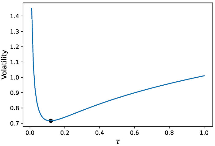
Fig.1: Volatility curve of a noisy fractional Brownian motion with 𝐻=0.75. The minimal volatility is marked with a black dot. Under the standard Brownian motion model, the volatility would be constant at all time scales.

We apply real-world data to estimate the volatility and Hurst exponents. Specifically, we consider a collection of exchange-traded funds (ETFs) and stocks (tickers: SPY, IWM, QQQ, XLK, AAPL, and MSFT), with dates ranging from January 2020 to February 2023. For our experiments, we use 3s high-frequency intraday price data. Prices are recorded on each day from open to close, spanning 6.5 hours, making 7800 equal-spaced time points. We choose a time frame such that 𝑡=1 corresponds to 1 min

Fig. 2. shows the multiscale volatility estimated on a 3s intraday price time series. We see that the volatility is clearly not constant across timescales. There is a consistent downward slope across all six tickers. For AAPL and MSFT, we see a clear sharp drop in volatility when the timescale is very small. This phenomenon matches the asymptotic behavior of the noisy fractional Brownian motion model, showing clear evidence of the microstructure noise. The finer sampling frequency may show a larger effect of the noise.

Fig 2: Volatility vs timescale, estimated from 3s intraday price data.

Next, we estimate the Hurst exponent for each intraday price path for every ticker.

The Hurst exponent is associated with the smoothness of the random process, long memory, and fractal dimension.

• When 𝐻=0.5, fBm reduces to the standard Brownian motion with independent increments.
• When 0<𝐻<0.5, the process is anti-persistent or mean-reverting with negatively correlated increments.
• When 0.5<𝐻<1, the process is persistent or trending with positively correlated increments.

Fig. 3 shows the histograms of daily Hurst exponent results, compared against the distribution of estimating the Hurst exponent from Brownian motion simulation. Although the Hurst exponent of the intraday data is centered around 1/2, we can clearly see that its distribution is not the same as Brownian motion.

Fig. 3: Hurst exponent estimated on 3 s intraday data from 2020 to 2023. This figure shows the histogram of the estimated values over all dates. The orange dash-line shows the distribution of the Hurst exponent estimator from a standard Brownian motion in comparison with that from the dataset.

The Hurst exponent H estimated on the real-world data is in general distributed to the left of a Brownian motion. The kernel density curves show a much wider spread distribution and feature long tails. There is a significant portion of days that have very low or high Hurst exponents, which is unlikely if the Brownian motion assumption holds.

This implies that the price dynamics can be different on different days. There are days when the price movement is mean-reverting, and on other days the movements are trending or like a random walk.

In reality, asset prices may exhibit patterns and seasonality of return distribution during trading hours. One well-known observation is the so-called U-shape volatility.

U-shape volatility: the volatility is highest near market open and close, and lowest at midday.

We show the intraday rolling Hurst exponent and noise level. TheHurst exponents vary at different times of day, i.e., the scaling exponent is not constant. For all of the tickers, the exponent is highest at market open, and then decreases rapidly.

Fig.4: The Hurst over a 1-hour rolling window from market open to market close. The x-axis marks the time of the day (e.g., 10 = 10 a.m. EST and 13 = 1 p.m. EST). The starting point of the window shifts on a 15 min basis. For each day, one rolling Hurst curve is estimated for each asset. The plot shows the average over all dates in the dataset.

Fig 5: The estimated microstructure noise level over a 1-hour rolling window from market open to market close. The x-axis marks the time of the day (e.g., 10 = 10 a.m. EST and 13 = 1 p.m. EST). The starting point of the window shifts on a 15 min basis. For each day, one rolling Hurst curve is estimated for each asset. The plot shows the average over all dates in the dataset.

Lastly, we show the 60-day rolling average of the Hurst exponent from 2020 to 2023. At the beginning of the pandemic in 2020, most assets have a Hurst exponent close to 0.5, corresponding to a random walk. The Hurst exponent then trends lower towards mean-reverting values and fluctuates for a period of time.

Overall, the ETFs tend to have a higher Hurst exponent, which stays closer to 0.5, while the Hurst exponent for the two stocks AAPL and MSFT tends to fluctuate below 0.5.

Fig 6: Time series of the Hurst exponent, realized volatility, and noise from 2020 to 2023. Values are estimated from intraday data sampled every 3 s for each ticker and averaged over 60-day rolling windows.

Educational purpose only. This is not investment advice. All returns are hypothetical.

Also read:

• High-Frequency Data source: https://www.kaggle.com/datasets/brtnsmth/intraday-market-data
• Multiscale Analysis & Volatility Asymmetry of Cryptocurrency Prices
• Multiscale Financial Signal Processing

Reference:

Leung, Tim, and Theodore Zhao. 2023. “Multiscale Volatility Analysis for Noisy High-Frequency Prices” Risks 11, no. 7: 117. https://doi.org/10.3390/risks11070117