An End to End Guide to Hyperparameter Optimization using RAPIDS and MLflow on Google’s Kubernetes Engine (GKE)

At the same time data science is becoming more tightly integrated into services and product development, we are also seeing a massive increase in both the scalability and compute power available from generational improvements in GPUs, and their availability in large scale cloud services, such as Google’s Kubernetes Engine (GKE). One major theme related to these changes is distributed Hyper-Parameter Optimization (HPO) for fine-tuning models in a massive and parallel fashion. Many of these changes will present a number of important considerations that will directly affect the speed, productivity, and functional interaction of teams within an organization.

First, it is increasingly important to be able to iterate quickly while making accurate predictions; workflows that used to run overnight or take days to complete, now span a coffee break or are bordering on interactive. Second, as our ability to run more experiments, faster, becomes a reality, we need to take a more structured approach to how we store, validate, and reproduce resulting work products. Third, we need to standardize the process of sharing these resulting artifacts between research, engineering, and operations teams. Lastly, we need to recognize and adapt to the operational challenges faced by business and academia in being able to effectively provide the necessary resources for actionable data science at scale.

This guide demonstrates how each of these challenges can be effectively addressed using a combination of:

1. RAPIDS for GPU accelerated Extract Transform Load (ETL) operations, and machine learning: RAPIDS provides much of the functionality of the traditional PyData infrastructure (Pandas, Scikit-Learn, NetworkX, etc..). As such, in most cases, it can be used as a drop-in replacement for its CPU-based counterparts. In this guide, we’ll leverage this to massively improve the training speed of HPO runs, utilizing NVIDIA’s Tesla T4 GPUs on the Google Kubernetes Engine (GKE) platform, and to exploit model compatibility with MLflow’s Scikit-Learn model registry extensions.
2. MLflow to enforce consistency, reproducibility, and a structured versioning process for models: MLflow allows for standardized workflows between research, engineering, and operations with the ability to track and publish RAPIDS based machine learning models while ensuring reproducibility. We will use these features to record all of the test parameters explored during a hyper-parameter optimization run and register the resulting ‘best’ model which can easily be deployed for inference.
3. Google’s Kubernetes Engine (GKE) to support ‘as needed’ hardware resource provisioning: Kubernetes is described as “an open source system for automating deployment, scaling, and management of containerized applications.” GKE provides a managed infrastructure that allows us to create on-demand clusters, deploy services, and directly run training jobs via MLflow. Kubernetes provides the flexibility necessary for modern organizations to support the large, distributed jobs often required by ML/DL workflows while balancing hardware allocations.

Our end result will be a GKE cluster deployment which:

1. Can easily be adapted for production environments; while we won’t go into configuring our services for high availability or secure authentication, these are standard use cases with well-known solutions processes that can be facilitated using GKE.
2. Will natively support GPU accelerated RAPIDS libraries; allowing us to run MLflow training jobs for RAPIDS models.
3. Hosts our own MLflow tracking server, leveraging a Postgresql database as a backing store, and Google Cloud Platform (GCP)’s gcsfs for artifact storage.

As a motivating example, we’ll build a random forest classifier utilizing the Airlines database (record of on-time performance statistics for U.S. airlines maintained by the U.S. Department of Transportation). For this process, we’ll also use Hyperopt, for Hyper-parameter Optimization (HPO), and record each of our experiments with MLflow. When finished, you will be able to predict whether or not a given flight will arrive ‘ON-TIME’, or ‘LATE’.

By the end of this guide, you will have a setup configured like the diagram below:

Cluster Diagram

RAPIDS Cloud Machine Learning Examples

This guide is built around the ‘mlflow’ example code found in the RAPIDS cloud-ml examples repo; all of the code and configuration scripts, referenced here, live in that repository.

To follow along:

git clone git@github.com:rapidsai/cloud-ml-examples.git
cd mlflow/docker_environment

Python Code

Before starting into how to configure your environment and spin up a GKE cluster, let’s take a look at the core python code used for training. This imports the required libraries define some helper functions to read data into a cuDF dataframe, and implements a simple training loop that Hyperopt will use to test parameters.

Imports

Imports

Everything here should be straight forward; cuDF and cuML are our GPU accelerated libraries equivalent to Pandas and Scikit-Learn; Hyperopt is our parameter optimization library, used to intelligently search our hyper-parameter space; gcsfs allows us to interact directly with our GCP storage bucket, and MLflow is used to record the results of our trial runs, and register the resulting best model.

Helper Functions

A simple data loader that reads a parquet file into a GPU dataframe, and a helper function that will read a file from gcsfs and write it to the local execution environment.

Training Loop

The training loop consists of a fairly standard ‘train’ function which will be called by hyperopt for every trial run. Train creates a nested MLflow run, so that each trial will be logged under the top-level experiment, logs the current configuration parameters, and then proceeds to train and evaluate a model.

Entrypoint Code

The entrypoint code does a few boilerplate operations, processing command arguments, and defining our HPO search space. Additionally, it’s also responsible for defining Hyperopt’s entrypoint function, starting our top-level parent run with MLflow, and registering a final model based on the optimal hyperparameters returned from Hyperopt. Here it is worth mentioning that we construct ‘fn’, the function passed to Hyperopt, utilizing python’s ‘partial’ library to facilitate passing static configuration data to our training routine.

Note that we use MLflow’s ‘sklearn.log_model’ interface to register our final model, even though our underlying model is implemented in RAPIDS. This is possible because RAPIDS is designed to provide a compatible interface with each of the PyData framework components for which it defines a GPU accelerated equivalent. What this means to an end-user is that, in most cases, you will be able to update your existing code to use RAPIDS, with minimal changes; often nothing more than an import statement.

Setup and Prerequisites

For the purposes of this example, we will assume that you are running commands from a workstation, running Python 3.7+, with a functioning Docker installation; you will also need a Kubernetes cluster, running in GKE, with an appropriately configured Kubectl, a GCP storage bucket, and GCR repository which are all accessible from your GKE cluster. Don’t worry if you don’t have the GCP/GKE elements at the moment, we’ll cover how to create and configure them below; additionally, you can refer to this detailed guide, for specifics with regard to each step.

There will be a number of parameters that you’ll use, that will be specific to your environment, these will be indicated as ‘VARIABLE_NAME’, and referenced in commands as linux style environment variables ‘${VARIABLE_NAME}’. Here are some of the initial parameters you’ll need to determine:

• YOUR_PROJECT: The name of the GCP project where your GKE cluster will live.
• YOUR_REPO: The name of the repository where your GCR images will live.
• YOUR_BUCKET: The name of the GCP storage bucket where your data will be stored.
• MLFLOW_TRACKING_UI: The URI of the tracking server you will deploy to your GKE cluster.

Local Environment

It is advisable to use a virtualized environment, such as Anaconda or VirtualEnv to isolate your python installation, but not required for this guide.

Software

• Install Docker
• Install Kubectl

Python Libraries

To ensure that you have a functional local environment that will be capable of running MLflow experiments, and interacting with your GKE cluster, you’ll need to install a few python libraries.

pip install mlflow, gcsfs, google-cloud, google-cloud-storage, kubernetes

Data

Download the training data, which consists of 20,000 rows and 14 columns, with columns consisting of data such as ‘origin’, ‘destination’, ‘carrier, and ‘trip distance’.

wget -N https://rapidsai-cloud-ml-sample-data.s3-us-west-2.amazonaws.com/airline_small.parquet

Verify columns and shape

python
>>> import cudf
>>> data = cudf.read_parquet(‘airline_small.parquet’)
>>> data.columns
Index(['ArrDelayBinary', 'Year', 'Month', 'DayofMonth', 'DayofWeek',
'CRSDepTime', 'CRSArrTime', 'UniqueCarrier', 'FlightNum',
'ActualElapsedTime', 'Origin', 'Dest', 'Distance', 'Diverted'],
dtype='object')
>>> data.shape
(200000, 14)

Post-GKE Configuration

Once your GKE environment is configured (see below), there is some additional work that needs to be done on your local system.

• Configure Kubectl to point at your new cluster, and verify it is working

kubectl get all
NAME                   TYPE         CLUSTER-IP       ....
service/kubernetes     ClusterIP    xxx.xxx.xxx.xxx  ....

• Authenticate Docker with your GCR account

gcloud auth login

GCP Environment

Storage

You’ll need to create a storage bucket that will act as both an artifact endpoint for MLflow, and as a central repository to store the training data that will be pulled by the MLflow workers.

Create a Service Account

• Create a keyfile, and save it as ‘keyfile.json’

Create a Storage Bucket

• Add the previously created service account as a ‘Storage Object Admin’ for your bucket.
• Add data and artifact storage paths to the storage bucket
• Create your MLflow artifact directory GS_ARTIFACT_PATH:
  ex. ‘gs://${YOUR_BUCKET}/artifacts’
• Upload airline_small.parquet you previously downloaded to (GS_DATA_PATH):
‘gs://${YOUR_BUCKET}/airline_small.parquet’
• Upload the conda.yaml, found here, to GS_CONDA_PATH:
‘gs://${YOUR_BUCKET}/conda.yaml’
• Decide on a GCR naming convention for images you’ll be creating/using, We’ll refer to this as GCR_REPO
  ex. ‘gcr.io/${YOUR_PROJECT}/${YOUR_REPO}

GKE Cluster

• Create your GKE cluster
• Once it is up and running, go to your GCP console, click on your cluster, and verify that you have an adequate number of CPU and GPU nodes available. For example:

• Install the NVIDIA driver installation daemonset.

Note: As of this writing, the most recent GKE version did not provide a CUDA 11 compatible driver; you will need to install it manually here, but this may not be required going forward. For more information, see here.

kubectl apply -f https://raw.githubusercontent.com/GoogleCloudPlatform/container-engine-accelerators/master/nvidia-driver-installer/cos/daemonset-nvidia-v450.yaml

Infrastructure deployment

GCP Authentication

Before we do anything else, we need to make sure that our services will be able to read and write to our storage bucket; for that, we’ll need to expose the keyfile.json file that we created, which holds the credentials for our service account! This will be mounted into our tracking server at /etc/secrets/keyfile.json.

kubectl create secret generic gcsfs-creds --from-file=./keyfile.json

MLflow

Next up, we need to deploy our MLflow tracking server, and a Postgresql service which will act as MLflow’s backing store. For each service, we’ll be using a predefined Helm chart, which essentially allows us to coalesce elements of a kubernetes deployment into a nice package and save time. I won’t go into great detail since they’re not directly relevant to this guide. If you want to learn more about Helm, check it out here.

Backing Store Deployment

This will install a Postgresql database in our cluster that will act as MLflow’s backing store. For this, we’ll just use Bitnami’s Helm Deployment.

helm repo add bitnami https://charts.bitnami.com/bitnami
helm install mlf-db bitnami/postgresql --set postgresqlDatabase=mlflow_db --set postgresqlPassword=mlflow \
--set service.type=NodePort

MLflow Tracking Service

This process has a few more steps, it will require you to:

• Build a new Docker container that will host our MLflow tracking service.
• Push this container to your GCR_REPO

Deploy the tracking service defined here, using Helm.

Building the tracking service

To build our tracking service, we’ll need two things: a Dockerfile, to define how to build the container, and an entrypoint script that launches the MLflow tracking service. As a reminder, each of these files can be found in the RAPIDS cloud examples repo on Github.

Dockerfile.tracking

This provides the bare minimum elements necessary to launch the MLflow tracking service, and ensure that it is able to talk to the GCP storage system (gcsfs)

Tracking Server Entrypoint

This entrypoint script gives us a simple, configurable way to launch the MLflow tracking service when the container is started.

Given these two components, we’re able to build our tracking service and push it to GCR.

docker build --tag ${GCR_REPO}/mlflow-tracking-server:gcp --file Dockerfile.tracking .
docker push ${GCR_REPO}/mlflow-tracking-server:gcp

Deploy the tracking service via Helm chart.

At this point, we’ve built the container that will host the tracking service and pushed it to GCR. All that’s left is to deploy it on our cluster.

cd helm
helm install mlf-ts ./mlflow-tracking-server \
  --set env.mlflowArtifactPath=${GS_ARTIFACT_PATH} \
  --set env.mlflowDBAddr=mlf-db-postgresql \
  --set service.type=LoadBalancer \
  --set image.repository=${GCR_REPO}/mlflow-tracking-server \
  --set image.tag=gcp

After launching the tracking service, we need to wait for the service to come up, and the load balancer to be assigned an external IP address, which will allow us to verify everything is working as expected.

watch kubectl get svc

Once the external IP is no longer pending, we’ll refer to it as MLFLOW_TRACKING_SERVER. To verify that the service is up and functioning correctly, open a browser window, and go to ‘https://${MLFLOW_TRACKING_SERVER}’. You should be presented with a clean MLflow tracking console interface that looks like this:

MLflow Clean Interface

If everything looks good so far, congratulations! Most of the hard work is over!

RAPIDS with MLflow Experiments, on Kubernetes

At this point, we have a fully configured GKE cluster, we have a tracking service with back end and artifact storage, and we have python training code. What’s left to do?

• Package our training code as an MLflow project.
• Build a container that MLflow will use to launch Kubernetes jobs.

Packaging our Code

A common problem that exists between research and development and the rest of an organization is communicating how to use the work they produce. A model will be created, and ‘thrown over the fence’ for engineering or ops to deploy into production; often without consistent documentation on how it should be used. This is undesirable and can lead to ad-hoc processes, poor model versioning and management, and an obscured understanding of how models were trained and validated.

MLflow offers a standardized solution to this workflow, in the form of ‘projects’ which create a common interface for training and deployment, and a backing store + model registry for tracking telemetry of the training process, as well as model versioning and storage. When taken together, these tools allow for situations where models can be trained in a reproducible manner and stored in a way that easily allows operations teams to select those ready for production use.

Projects are defined via a simple wrapper format, shown below. For more information, see the MLproject specification.

MLProject Definition

Above, we define a simple MLproject specification called ‘cumlrapids’, that declares that it will run as a docker environment, using the ‘rapids-mlflow-training:gcp’ container. The project declaration also defines an entrypoint template called ‘hyperopt’, which defines how the command should be executed in the training container.

Building a Training Container

Next, we need to create a Dockerfile that will be used to build the ‘rapids-mlflow-container:gcp’ container declared in the MLproject file. This process follows the same steps used previously to construct our tracking server container.

Again, we define a minimal set of dependencies that supports our training code. In this case, we’ll use the latest release version of RAPIDS, utilizing python 3.8, and CUDA 11, and install any additional libraries required to interact with GCP and MLflow.

Training Entrypoint

Here, we define the entrypoint that will be called by MLflow when launching new training jobs. Something to note here is that we use this entrypoint.sh script to proxy any commands passed to the container; it will first activate the ‘rapids’ conda environment, and then launch the training script prescribed in the MLproject file.

Using these two scripts, we can build our training container, and prepare to launch experiments.

docker build --tag rapids-mlflow-training:gcp --file Dockerfile.training .

Launch an HPO Training Experiment

Point MLflow at our tracking service

export MLFLOW_TRACKING_URI=http://${MLFLOW_TRACKING_URI}

Edit k8s_config.json, and set the repository-uri field to use your GCR_REPO, for example:

{
  "kube-context": "",
  "kube-job-template-path": "k8s_job_template.yaml",
  "repository-uri": "${GCR_REPO}/rapids-mlflow-training"
}

At this point, we are ready to launch training runs, which will be logged to our tracking server, and register the resulting RAPIDS RandomForest model within the MLflow model registry.

mlflow run . --backend kubernetes \
  --backend-config ./k8s_config.json -e hyperopt \
  --experiment-name RAPIDS-MLFLOW-GCP \
  -P conda-env=${GS_CONDA_PATH} -P fpath=${GS_DATA_PATH}

This will launch a new training run in our GKE cluster, log all of the expected telemetry with our tracking server, and then save and register a model utilizing the best-identified parameters.

Note: This process can take some time on the first run, around 5 to 10 minutes; this is because MLflow will need to construct a new container by injecting all the necessary project code into the ‘rapids-mlflow-training’ container created earlier, and push it to GCR. Subsequently, each worker will need to pull the container to its local file system when running the training code. After this initial lagged deployment, all additional runs will start almost instantaneously.

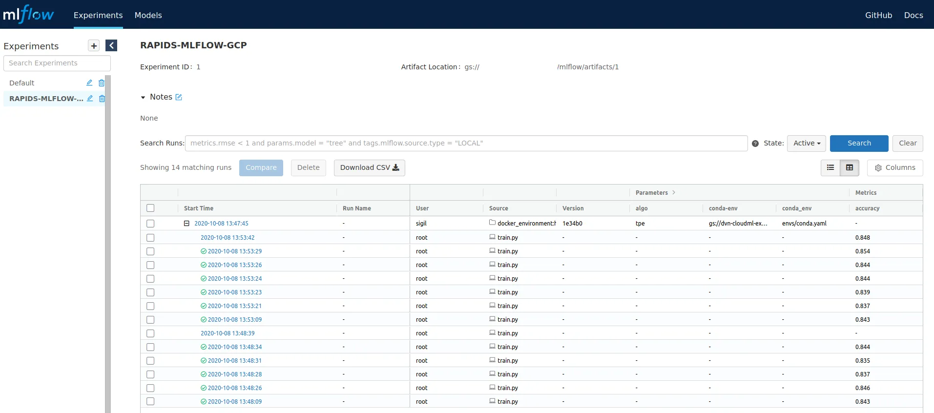
After the experiment runs complete, you can again point your browser at the MLflow tracking server, and view the resulting training logs, as seen below.

MLflow HPO Tracking Run

MLflow Registered Model

Conclusion

If you’ve made it to this point, congratulations! You have all the components required to train, record, and register GPU accelerated machine learning models, using RAPIDS and MLflow on your own Kubernetes cluster.

To recap what you’ve done so far:

• Configured your own GKE cluster, with GCP based storage.
• Deployed a fully functional cluster to support RAPIDS + MLflow based workflows.
• Wrapped an example RAPIDS based machine learning project, with an MLProject interface.
• Launched a GPU accelerated Hyper-Parameter Optimization (HPO) training run, using MLflow.

Quite an achievement!

Additionally, while this particular deployment does not address things like high availability, or security, it does provide a baseline, utilizing standard tools, which can be extended to support these production use cases in your environments.

I hope this guide has been helpful! Please keep an eye out for what comes next, or leave feedback regarding the RAPIDS based use cases you’d like to see.

For more information about the technologies we’ve used, such as RAPIDS, MLflow, Hyperopt (or HPO in general), Kubernetes, or Helm, see the following links:

RAPIDS

Open GPU Data Science | RAPIDS

RAPIDS + HPO | RAPIDS

RAPIDS Github

MLflow

MLflow - A platform for the machine learning lifecycle

Hyper-Parameter Optimization

Ax · Adaptive Experimentation Platform

Hyperopt Documentation

Optuna - A hyperparameter optimization framework

Kubernetes

Production-Grade Container Orchestration

Helm