2D Mapping using Google Cartographer and RPLidar with Raspberry Pi

Published in

Robotics Weekends

7 min readOct 12, 2020

In this experiment I’m going to launch opensource SLAM software — Google Cartographer — on Raspberry Pi b3+ with 360 degrees LDS RPLidar A1m8

All the SLAM process is launched on the Raspberry PI. Cartographer is configured to use only Lidar data for map building and position estimation. No IMU is used.

I assume that you have Ubuntu 18.04 and ROS already installed on your Raspberry Pi.

This is a more detailed description and answers to questions in comments for the video published on Robotics Weekends YouTube channel.

What is Google Cartographer

Cartographer is a system that provides real-time SLAM (simultaneous localization and mapping. In other words using information from lidar and other sensors Cartographer can build a map of environment and show where robot is located related to the map. Cartographer can build maps in 2D and 3D. But for 3D map Pointcloud as a source is needed. We are going to use RPLIDAR a1m8 as a main sensor. This sensor provides 360 degree distance measurements as a thin line — Laserscan.
Cartorgapher supports multiple lidars, IMUs and other approaches to increase SLAM quality. But the minimum sensor set is a single 360 degree LDS sensor (RPLIDAR in our case), and I’m going to test how it works.
Cartographer has a ROS integration package — cartographer_ros. You can build it from source or get from the ROS repository. For the first try I’d recomment a second option.

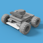
3D printed parts

To make experiment more convenient I’ve printed several parts to hold RPLIDAR, Raspberry Pi and powerbank together. You can download STL files from Thingiverse

The whole device consists of RPLIDAR as a sensor, Raspberry Pi as a computer, and powerbank as a power source. Assembled device is rather simple and solid:

Explaining software part

Below you can see a high level description of the entire setup. RPLIDAR is connected to the Raspberry Pi, Cartographer is installed and running on Raspberry Pi, laptop is used for visualization.

As I’m using headless system on Raspberry Pi (without GUI), visualization will be performed on laptop. Laptop also has ROS installed.
To configure ROS to work through the network you have to specify two Environment Variables: ROS_IP and ROS_MASTER_URL on both computers. You can find detailed information in ROS Wiki.

Raspberry Pi

Note — I assume that you have already installed Ubuntu on Raspberry Pi and installed ROS Melodic.
First you have to install Cartographer and rplidar ROS package:

sudo apt install ros-melodic-cartographer-ros ros-melodic-rplidar-ros

After the package is installed, create catkin workspace and clone gbot_core package from Github into src directory:

git clone https://github.com/Andrew-rw/gbot_core.git

The package does not contain any code to compile, but has configuration files and launch scripts important for SLAM system. Let’s take a look at them in detail.
In configuration_files directory you can find a configuration for Cartographer:

include "map_builder.lua"
include "trajectory_builder.lua"options = {
  map_builder = MAP_BUILDER,
  trajectory_builder = TRAJECTORY_BUILDER,
  map_frame = "map",
  tracking_frame = "base_link",
  published_frame = "base_link",
  odom_frame = "odom",
  provide_odom_frame = true,
  publish_frame_projected_to_2d = true,
  use_odometry = false,
  use_nav_sat = false,
  use_landmarks = false,
  num_laser_scans = 1,
  num_multi_echo_laser_scans = 0,
  num_subdivisions_per_laser_scan = 1,
  num_point_clouds = 0,
  lookup_transform_timeout_sec = 0.2,
  submap_publish_period_sec = 0.3,
  pose_publish_period_sec = 5e-3,
  trajectory_publish_period_sec = 30e-3,
  rangefinder_sampling_ratio = 1.,
  odometry_sampling_ratio = 1.,
  fixed_frame_pose_sampling_ratio = 1.,
  imu_sampling_ratio = 1.,
  landmarks_sampling_ratio = 1.,
}MAP_BUILDER.use_trajectory_builder_2d = trueTRAJECTORY_BUILDER_2D.min_range = 0.5
TRAJECTORY_BUILDER_2D.max_range = 8.
TRAJECTORY_BUILDER_2D.missing_data_ray_length = 8.5
TRAJECTORY_BUILDER_2D.use_imu_data = false
TRAJECTORY_BUILDER_2D.use_online_correlative_scan_matching = true
TRAJECTORY_BUILDER_2D.real_time_correlative_scan_matcher.linear_search_window = 0.1
TRAJECTORY_BUILDER_2D.real_time_correlative_scan_matcher.translation_delta_cost_weight = 10.
TRAJECTORY_BUILDER_2D.real_time_correlative_scan_matcher.rotation_delta_cost_weight = 1e-1
TRAJECTORY_BUILDER_2D.motion_filter.max_angle_radians = math.rad(0.2)
-- for current lidar only 1 is good value
TRAJECTORY_BUILDER_2D.num_accumulated_range_data = 1POSE_GRAPH.constraint_builder.min_score = 0.65
POSE_GRAPH.constraint_builder.global_localization_min_score = 0.65
POSE_GRAPH.optimization_problem.huber_scale = 1e2
POSE_GRAPH.optimize_every_n_nodes = 35return options

Most of the parameters were obtained experimentally or calculated according to RPLIDAR’s specification, but some of them I’d like to highlight. As the only sensor we are going to use is RPLIDAR, localization will be calculated from spatial difference between scanned data and a calculated map, built from previous scans. So Cartographer will be a source of odometry.
Parameter provide_odom_frame = true means that Cartographer will publish transforms between published_frame and map_frame. In our case it will be TF transform between “base_link” and “map”.
Parameter publish_frame_projected_to_2d = true means that published transforms will be only in X and Y coordinates, no elevations exist.
Parameter use_odometry = false means that there are no other odometry sources. Cartographer will just stick “odom” frame to “map”. Again, for our simple case it is fine.
TRAJECTORY_BUILDER_2D.use_imu_data = false says that we won’t use IMU and count only on Laserscan points matching algorithm.
More information about specific parameters you can find in Cartographer documentation.
In the rviz directory there is a RViz view file with the list of already set up topic listeners, to make mapping visualization more convenient to use.
In the urdf directory there is a so-called robot description — file which contains a robot’s physical description to ROS. There is information like sensors’ spatial position and relations, joints’ type, length, mass, inertia, etc. More information is on ROS Wiki page. For our test bench creating URDF is an overhead— there is only one link between base and lidar and it could be added to the launch file as a static transform — but this file is a good starting point if you decide to add an IMU sensor, range finders or something else. URDF description language is build on top of XML:

<robot name="head_2d">  <material name="orange">
    <color rgba="1.0 0.5 0.2 1" />
  </material>
  <material name="gray">
    <color rgba="0.2 0.2 0.2 1" />
  </material>  <link name="laser">
    <visual>
      <origin xyz="0 0 0" />
      <geometry>
        <cylinder length="0.03" radius="0.03" />
      </geometry>
      <material name="gray" />
    </visual>
  </link>  <link name="base_link">
    <visual>
      <origin xyz="0.01 0 0.015" />
      <geometry>
        <box size="0.11 0.065 0.052" />
      </geometry>
      <material name="orange" />
    </visual>
  </link>  <joint name="laser_joint" type="fixed">
    <parent link="base_link" />
    <child link="laser" />
    <origin rpy="0 0 3.1415926" xyz="0 0 0.05" />
  </joint></robot>

And finally, in the launch directory there are two scripts which are used for starting SLAM process (gbot.launch) and starting visualization (visualization.launch). Structure of gbot.launch is simple enough — first is starting robot description node, then Lidar and at the end — Cartographer. The last node, cartographer_occupancy_grid_node, is used for conversion of Cartographer map data to more popular in ROS navigation stack Occupancy Grid. Occupancy Grid represents the environment as a grid of cells where each cell holds a probability value that the cell is occupied in the range [0,100]. This launch file should be executed on the Raspberry Pi.

<launch>
  <!-- Load robot description and start state publisher-->
    <param name="robot_description" textfile="$(find gbot_core)/urdf/head_2d.urdf" /><node name="robot_state_publisher" pkg="robot_state_publisher" type="robot_state_publisher" />
  
  <!-- Start RPLIDAR sensor node which provides LaserScan data  -->
    <node name="rplidarNode" pkg="rplidar_ros" type="rplidarNode" output="screen">
        <param name="serial_port" type="string" value="/dev/ttyUSB0"/>
        <param name="serial_baudrate" type="int" value="115200"/>
        <param name="frame_id" type="string" value="laser"/>
        <param name="inverted" type="bool" value="false"/>
        <param name="angle_compensate" type="bool" value="true"/>
    </node>
  
  <!-- Start Google Cartographer node with custom configuration file-->
    <node name="cartographer_node" pkg="cartographer_ros" type="cartographer_node" args="
          -configuration_directory
              $(find gbot_core)/configuration_files
          -configuration_basename gbot_lidar_2d.lua" output="screen">
    </node><!-- Additional node which converts Cartographer map into ROS occupancy grid map. Not used and can be skipped in this case -->
    <node name="cartographer_occupancy_grid_node" pkg="cartographer_ros" type="cartographer_occupancy_grid_node" args="-resolution 0.05" />
    
</launch>

Structure of visualization.launch is even simpler. The purpose of it is to start rviz with prepared view configuration.

<launch>
  <!-- Start RViz with custom view -->
  <node pkg="rviz" type="rviz" name="show_rviz" args="-d $(find gbot_core)/rviz/demo.rviz"/>    
</launch>

Laptop

To visualize Carographer data properly cartographer-rviz package should be installed on laptop:

sudo apt install ros-melodic-cartographer-rviz

To be able to launch visualization script I recommend to clone gbot_core on laptop also.
And just to note - Cartographer and visualization can be launched from a single computer without any changes in configuration.

Cartographer testing

Well, assuming than network connection between computers is established, we are ready to start the Cartographer and visualization nodes.
On Raspberry Pi launch mapping process:

roslaunch gbot_core gbot.launch

You should see a similar response in terminal:

Then on laptop (or just in a separate terminal, if you are using same PC) start visualization:

roslaunch gbot_core visualization.launch

The result should be a started RViz:

RViz rendering Cartographer’s Submaps data

During moving the lidar around the room map will become more detailed and with higher and higher contrast. It means that Cartographer’s uncertainty about the environment decreases. Also you will see a trajectory as a blue line, extracted from calculated odometry:

Conclusion

Cartographer can provide 2D odometry of decent quality, by using only low cost 360 degree LDS with pretty low data rate (5–7 Hz).
IMU and additional odometry source (for example wheeled platform odometry or visual odometry) can increase resulting map quality on big environment areas. But for indoor mapping of about 50–60 square meters area they are not so important — Cartographer’s internal loop closure algorithm is capable of keeping such small maps consistent.

Thank you

I would like to thank Arbitrary Constant and Doina Moga for inspiring and supporting me to finish this story.

Links

3D files: https://www.thingiverse.com/thing:3970110
Project on GitHub: https://github.com/Andrew-rw/gbot_core
Cartographer Wiki: https://google-cartographer.readthedocs.io/en/latest/
YouTube video: https://youtu.be/qNdcXUEF7KU