Summary Of Deep Learning With Differential Privacy

First why this paper ?
I assume you have some sort of background in Machine Learning.
As we can see in today’s world , Machine learning Algorithms are being applied on variety of problems specifically including the ones which relates to big data and its analysis.
But as more and more problems are solved through machine learning algorithms , it also includes large datasets often involving sensitive data and by sensitive i mean it may contain some really sensitive data specially which are organised through crowdsourcing.

The idea is that the model should not reveal any private information about a particular individual whether he participated in a study or not.
Let’s understand the importance of differentially private mechanism required today through some examples :
- ➡️ So, let’s say a data analyst crowdsourced a dataset and publicized it as a method for helping them to find about a particular kind of disease so that their organisation can create specific medicine for that ( say , Cancer or AIDS) which people not wanna tell to anyone. But what if the trusted curator (here , data analyst) wants to obtain some specific info about a individual or what if a attacker intrudes and identifies a person whether he is suffering from that disease or not ? What kind of harm will he have if the attacker reveals the info in public ?
- ➡️ There is a nationwide identity card issue to people in India named as “Aadhar Card” which publicizes itself as identity card for type of work or permit. Now the kind of information your aadhar bio data helds is really very sensitive like your iris scan , your fingerprints and other info which you might not wanna tell to someone but due to pressure you have to register for it. What kind of harm will a person have if that personal body signatures are revealed in public or to any attacker ?
What the paper wants to acheive ?
- 👉 In the paper, researchers aim to combine state-of-the-art machine learning methods with advanced privacy-preserving mechanisms, training neural networks within a modest (“single-digit”) privacy budget.
- 👉 Demonstrate that, by tracking detailed information (higher moments) of the privacy loss, one can obtain much tighter estimates on the overall privacy loss, both asymptotically and empirically. We improve the computational efficiency of differentially private training by introducing new techniques.These techniques include efficient algorithms for computing gradients for individual training examples, subdividing tasks into smaller batches to reduce memory footprint, and applying differentially private principal projection at the input layer.
- 👉 The Implementation is on the machine learning framework Tensor- Flow for training models with differential privacy. The two important datasets that has been used here are ‘MNIST’ and ‘CIFAR-10’ which are also the longest serving benchmarks for machine learning algorithms.
The algorithm which is described in the paper is used against strong adversary which has full knowledge of training mechanism and model parameters , which makes it really attractive piece of paper to study.
This makes it particulary useful for applications of machine learning on mobile devices, phones , tablets 📲 💻
Storing the models on device enables power-efficient, low-latency inference, and may contribute to privacy since inference does not require communicating user data to a central server.
Some background for Differential privacy and Deep learning :
According to Cynthia Dwork :
“Differential privacy” describes a promise, made by a data holder, or curator, to a data subject: “You will not be affected, adversely or otherwise, by allowing your data to be used in any study or analysis, no matter what other studies, data sets, or information sources, are available.”
let’s talk a bit about formal definition of differential privacy —

A randomized algorithm M with domain N ^ |X| is (ε, δ)-differentially private if for all S ⊆ Range(M) and for all x, y ∈ N |X| such that ∥x − y∥1 ≤ 1 if satisfies the above constraint , then it is said to be differentially private.
Basically , the above definition gives us an quantitative idea of how should a algorithm must work in order to be different private and quantifies our privacy loss on a database.
If δ = 0, M is ε-differentially private.
In case of (ε, δ) differentially private mechanisms , there is a little possibility that a attacker can find out info about a particular individual (though very rare chance) , whereas it is not same in (ε, 0) -differentially private.
Let’s understand a little about senstivity —
sensitivity is said to be maximum change in the output of query of a function when we remove one of the instances from the database (that is all the information related to one specific person).
Mathematically,

It is defined in terms of L1 norm.
Typically we are interested in values of δ that are less than the inverse of any polynomial in the size of the database. In particular, values of δ on the order of 1/∥x∥1 are very dangerous: they permit “preserving privacy” by publishing the complete records of a small number of database participants.

Generally noise is added when we make queries on database to make statistical analysis of the data , and there are several types of noise mechanism , one of which is gaussian mechanism.

Deep learning systems have been able to remarkably acheive state-of-the-art performance in many engineering applications.
But what makes it remarkably special ?
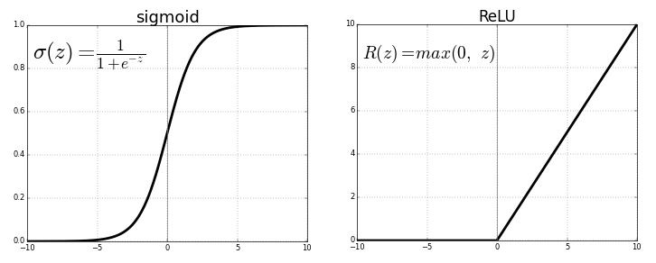
Basically , DL models are effective at finding non linear boundaries by fitting any given set of input/output examples by using activations functions , more used of them are ReLU’s and sigmoids.

So , say we need to classify on a training data which consists of cats and dogs , and given a image , we need to predict if it’s a cat or a dog.
So , we need to first predict the probability by passing our input data to model and then we need to define a loss function ‘L(θ)’ which represents the penalty for mismatching the training data. The loss ‘L’ on parameters θ is the average of the loss over the training examples {x₁, . . . , xₙ }.
Main aim is to find the global minima by updating the parameters and move in the negative direction of gradient.
Then we update the weights and bias of the network so that we get better prediction. This is also known as backpropogation algorithm.
In practice due to memory and other constraints , we need to perform gradient descent by mini-batch stochastic gradient descent (SGD) algorithm. In this algorithm, at each step, one forms a batch B of random examples and computes the loss over at entire mini batch and then updates the parameters.
This is generally effective for long run of models .
This following paper we are going through is based and using TensorFlow , an opensource dataflow engine released by Google.
Let’s now go on to understand main components of the approach described by this paper.
Differentially Private SGD Algorithm :
There are many ways to protect the privacy of the data using algorithms which attempts by working on final parameters that result from training process , treating this process as a black box.
But this paper describes a algorithm which applies more sophisticated approach in which the aim is to control the influence of the training data during the training process, specifically in the SGD computation , although this technique has been earlier used , but there has been several modifications and extensions in particularly , in the privacy accounting.

Description of algorithm :
Algorithm 1 outlines our basic method for training a model with parameters θ by minimizing the empirical loss function L(θ). At each step of the SGD, we compute the gradient ∇θL(θ, xi) for a random subset of examples, clip the l2 norm of each gradient, compute the average, add noise in order to protect privacy, and take a step in the opposite direction of this average noisy gradient. At the end, in addition to outputting the model, we will also need to compute the privacy loss of the mechanism based on the information maintained by the privacy accountant.
🤔 Okay don’t be overwhelmed 😞. So, let’s go one by one —
First you can see we have our inputs or examples as {x₁, . . . , xₙ}
Next we define a loss function and remember this loss is taken averaged on all the examples.
Next, hyperparameters : learning rate ηt , noise scale σ , group size L , gradient norm bound C.
⬛ First we initialize the parameters θ₀ (weights and biases)
⬛ next , we loop for training the model (epochs) -
👉 Now we first take a random sample Lₜ with probability L/N
👉Compute the gradient — that is derivative of loss function with respect to its inputs and parameter.
👉 Now , comes clipping the gradient. Let’s understand this.
It is possible for the updates to the weights to be so large that the weights either overflow or underflow their numerical precision.
This starts the process called gradient explosion as the unstable training process causes the network to fail to train in such a way that the model is essentially useless.
We have a solution — Gradient clipping involves forcing the gradient values (element-wise) to a specific minimum or maximum value if the gradient exceeded an expected range.
Let’s focus on the following term :

Since there is no bounding on the gradient , we will clip each gradient in l₂ norm.
To make it in the useful range , we apply clipping as shown in above picture.
Let’s take a example -
Say we have threshold C = 10 and say gradient calculated is (g) = 5 , then we see that g < C , so max(1, ||g||₂ / C) = max(1, 0.5) will return 1 and therefore , g is preserved (same as before).
But let’s say g = 200 , then we see that g > C , max(1, ||g||₂ / C) = max(1, 20) will return 20 and gradient is clipped accordingly as g <- g/20 which brings it to required range to avoid gradient explosion.
👉 Then we add the noise to the gradient calculated calculated over the the lots (The average provides an unbiased estimator, the variance of which decreases quickly with the size of the group. We call such a group a lot, to distinguish it from the computational grouping that is commonly called a batch).
👉 Finally , we take the gradient descent step in the negative of direction of gradient calculated to move our objective function towards global minima.
Now , the output is final model parameters and the overall privacy cost (ε, δ) using a method known as privacy accounting method which we will see soon.
Privacy accounting: For differentially private SGD, an important issue is computing the overall privacy cost of the training. The composability of differential privacy allows us to implement an “accountant” procedure that computes the privacy cost at each access to the training data, and accumulates this cost as the training progresses. Each step of training typically requires gradients at multiple layers, and the accountant accumulates the cost that corresponds to all of them.
Moment accounting : The moments accountant keeps track of a bound on the moments of the privacy loss random variable (defined below in Eq. (1)). It generalizes the standard approach of tracking (ε, δ) and using the strong composition theorem.

Next see the equation which is very close to defining the privacy loss in sens of differential privacy :

and the moment :

Hyperparameter Tuning :
One of the important things in deep learning models is hyperparameter tuning because without it , one can’t acheive higher accuracy and considerably low loss indicating minima for objective function (loss function).
In the paper, the effort is that we can tune hyperparameters in order to balance privacy, accuracy, and performance. In particular, through experiments, it is observed that model accuracy is more sensitive to training parameters such as batch size and noise level than to the structure of a neural network.
Let’s go one by one :
👉 Batch size and epochs :
While differentially private optimization of convex objective functions is best achieved using batch sizes as small as 1, non-convex learning, which is inherently less stable, benefits from aggregation into larger batches. At the same time, Theorem 1 suggests that making batches too large increases the privacy cost, and a reasonable tradeoff is to take the number of batches per epoch to be of the same order as the desired number of epochs.
👉 learning rate :
The learning rate in non-private training is commonly adjusted downwards carefully as the model converges to a local optimum. In contrast, we never need to decrease the learning rate to a very small value, because differentially private training never reaches a regime where it would be justified. On the other hand, in the experiments, it’s find that there is a small benefit to starting with a relatively large learning rate, then linearly decaying it to a smaller value in a few epochs, and keeping it constant afterwards.
Implementation of algorithm:
For actual source code you can go to this link.
For our purposes I attached a snippet (also shown in the paper) :

Experimental Results:
The results have been analysed on the two most popular datasets — MNIST and CIFAR - 10.
Okay before moving on , we fix some of the values which we will using to calculate moments accountant and privacy loss :
we set q = 0.01, σ = 4, and δ = 10−5 , and compute the value of ε as a function of the training epoch E.

Now we will start with each of the dataset and compare our results for baseline model and then differentially private model :
Baseline model : baseline model uses a 60-dimensional PCA projection layer and a single hidden layer with 1,000 hidden units. Using the lot size of 600, we can reach accuracy of 98.30% in about 100 epochs.
Differentially private model : For the differentially private version, we experiment with the same architecture with a 60-dimensional PCA projection layer, a single 1,000-unit ReLU hidden layer, and a lot size of 600. To limit sensitivity, we clip the gradient norm of each layer at 4. We report results for three choices of the noise scale, which we call small (σ = 2, σp = 4), medium (σ = 4, σp = 7), and large (σ = 8, σp = 16). Here σ represents the noise level for training the neural network, and σp the noise level for PCA projection. The learning rate is set at 0.1 initially and linearly decreased to 0.052 over 10 epochs and then fixed to 0.052 thereafter.


There has been lot of experiments by changing different hyperparameters one at a time , therefore We are going to see all the different results below :

Baseline model : We use the network architecture from the TensorFlow convolutional neural networks tutorial [2]. Each 32 × 32 image is first cropped to a 24 × 24 one by taking the center patch. The network architecture consists of two convolutional layers followed by two fully connected layers. The convolutional layers use 5 × 5 convolutions with stride 1, followed by a ReLU and 2 × 2 max pools, with 64 channels each. Thus the first convolution outputs a 12 × 12 × 64 tensor for each image, and the second outputs a 6×6×64 tensor. The latter is flattened to a vector that gets fed into a fully connected layer with 384 units, and another one of the same size. This architecture, non-privately, can get to about 86% accuracy in 500 epochs.
Differentially private version: For the differentially private version, we use the same architecture. As discussed above, we use pre-trained convolutional layers. The fully connected layers are initialized from the pre-trained network as well. We train the softmax layer, and either the top or both fully connected layers. Based on looking at gradient norms, the softmax layer gradients are roughly twice as large as the other two layers, and we keep this ratio when we try clipping at a few different values between 3 and 10. The lot size is an additional knob that we tune: we tried 600, 2,000, and 4,000. With these settings, the per-epoch training time increases from approximately 40 seconds to 180 seconds.
Now results for CIFAR 10:

Conclusions from the research:
Excerpt taken from paper :
We demonstrate the training of deep neural networks with differential privacy, incurring a modest total privacy loss, computed over entire models with many parameters. In our experiments for MNIST, we achieve 97% training accuracy and for CIFAR-10 we achieve 73% accuracy, both with (8, 10 ⁻⁵ )-differential privacy. Our algorithms are based on a differentially private version of stochastic gradient descent; they run on the TensorFlow software library for machine learning. Since our approach applies directly to gradient computations, it can be adapted to many other classical and more recent first-order optimization methods, such as NAG , Momentum , AdaGrad , or SVRG . A new tool, which may be of independent interest, is a mechanism for tracking privacy loss, the moments accountant. It permits tight automated analysis of the privacy loss of complex composite mechanisms that are currently beyond the reach of advanced composition theorems.
References :
Although the paper itself references various sources but here i am simply giving the link which contains the original paper and the sources :
🔗 https://arxiv.org/pdf/1607.00133.pdf
[Citations : arXiv:1607.00133v2 [stat.ML] 24 Oct 2016 ]
Authors : Martín Abadi∗ Andy Chu∗ Ian Goodfellow† H. Brendan McMahan∗ Ilya Mironov∗ Kunal Talwar∗ Li Zhang∗
∗Google. †OpenAI. Work done while at Google
— — — — — — — — — — — — — — — — — — — — — — — -
images : copyright reserved with their respective owners.
For more such awesome stories , you can subscribe or follow me.
Feel free to share your insights on the paper summary in the comments section below.
Clap it! Share it! Follow Me !
— — — — — — — — — — — — — — — — — — — — — — — —

— — — — — — — — — — — — — — — — — — — — — — — —
