Deep dive into the internals of Snowflake Virtual Warehouses
Snowflake’s Data Cloud provided as Software-as-a-Service (SaaS), enables data storage, processing, analytic solutions, Machine Learning, and running apps & services in a performant, easy-to-use, and flexible manner using “virtual warehouses” which is the primary compute primitive in Snowflake. This post details the internals of virtual warehouses which provide elastic, highly available, and fully managed mechanisms to run a variety of customer workloads on multiple cloud service providers.
Virtual Warehouse basics
Snowflake’s pioneering architecture that disaggregates compute from persistent storage enables independent scaling of both.
Virtual Warehouses are the primary compute primitive in Snowflake and are Massively Parallel Processing (MPP) compute clusters composed of multiple Virtual Machines (VMs) provisioned by Snowflake and run software managed by Snowflake. Virtual Warehouses provide elastic scaling, an instant-on experience, scale up & out, and automatically suspend & resume nearly instantly. VMs that comprise a warehouse cluster are interconnected to share data during job execution; compute clusters in a virtual warehouse do not share resources, which results in strong performance and resource isolation.

Virtual Warehouses consume billable compute as Snowflake credits on a per-second granularity as they execute jobs, load data, and perform other DML operations. One Snowflake credit represents the compute capacity to run a single-VM standard warehouse for one hour. A customer’s spend is a function of the size of the virtual warehouse and how long it runs. Virtual warehouses are only billed while they are started; when suspended, they are not billed.
Design tenets
The three primary tenets that have informed our approach with virtual warehouses include:
1/ To the extent possible, avoid presenting customers with choices and take on the often difficult work of assessing what is best for a given use case.
2/ Only show metrics around utilization and load that are actionable by customers.
3/ Preserve the flexibility to change attributes associated with underlying compute artifacts (e.g., VM SKU, shapes, size, counts, etc.) that back virtual warehouses behind the scenes.
Virtual Warehouse sizes and types
The warehouse type determines memory-to-CPU ratio of the virtual warehouse, while the size determines the total amount of CPU and memory available. There are two warehouse types (Standard and high-memory, branded as Snowpark-optimized) and multiple T-shirt sizes (XS, S, M, L, XL, … 6XL). Customers can modify the virtual warehouse size and type, even while it is currently executing queries.
Today, customers need to translate the criteria they reason about such as workload (as a collection of queries), desired completion time for the workload (a.k.a Service Level Objective), and cost budget into appropriate knob settings for compute capacity (via settings for warehouse size, warehouse type, cluster counts, scaling policy, etc.).
Memory spilling to inform warehouse type
The Snowpark-optimized warehouses type (which can help unlock ML training and memory-intensive analytics use cases) provides 16x more memory and 10x more local SSD cache per VM compared to standard warehouses. The larger memory speeds up computations while larger local storage provides speedup when cached intermediate results and artifacts such as Python packages and JARs are reused on subsequent runs.
When execution artifacts in Snowflake perform write operations of intermediate data, first, main memory on the virtual warehouse VMs are used; if this memory is full, data is “spilled” to local disk/SSD on virtual warehouse VMs — this is detailed in a subsequent section on storage architecture.
For performance-critical workloads, customers can choose larger warehouse sizes to ensure that the intermediate data fits in memory, or at least in disk, and does not spill to object storage (e.g., S3 on AWS).
Metrics exposed under the QUERY_HISTORY view such as BYTES_SPILLED_TO_LOCAL_STORAGE and BYTES_SPILLED_TO_REMOTE_STORAGE indicate the extent of memory pressure, which in many cases, can be addressed in a cost-efficient manner by moving to Snowpark-optimized warehouses of the same size.
The following query lists queries & warehouses that can benefit from increased size or by changing warehouse type to Snowpark-optimized.
SELECT QUERY_ID
 ,USER_NAME
 ,WAREHOUSE_NAME
 ,WAREHOUSE_SIZE
 ,BYTES_SCANNED
 ,BYTES_SPILLED_TO_REMOTE_STORAGE
 ,BYTES_SPILLED_TO_REMOTE_STORAGE / BYTES_SCANNED AS SPILLING_READ_RATIO
 FROM "SNOWFLAKE"."ACCOUNT_USAGE"."QUERY_HISTORY"
 WHERE BYTES_SPILLED_TO_REMOTE_STORAGE > BYTES_SCANNED * 5 - Each byte read was spilled 5x on average
 ORDER BY SPILLING_READ_RATIO DESC
 ;
The following query identifies the top 10 worst offending queries in terms of bytes spilled to local and remote storage.
SELECT query_id, SUBSTR(query_text, 1, 50) partial_query_text, user_name, warehouse_name,
 bytes_spilled_to_local_storage, bytes_spilled_to_remote_storage
 FROM snowflake.account_usage.query_history
 WHERE (bytes_spilled_to_local_storage > 0
 OR bytes_spilled_to_remote_storage > 0 )
 AND start_time::date > dateadd('days', -45, current_date)
 ORDER BY bytes_spilled_to_remote_storage, bytes_spilled_to_local_storage DESC
 LIMIT 10;
For performance-critical workloads, customers can choose larger warehouse sizes to ensure that the intermediate data fits in memory, or at least in disk, and does not spill to object storage (e.g., S3 on AWS).
Multi-cluster Warehouses
With multi-cluster warehouses, Snowflake supports allocating, either statically or dynamically, additional clusters to make a larger pool of compute resources available to the same virtual warehouse to increase job concurrency without managing multiple distinct virtual warehouses. To use this capability, customers can specify a minimum and maximum number of clusters for a given virtual warehouse.
While warehouse size & type scales a warehouse “up” and increases single-query performance, using multiple clusters in the same warehouse helps with query concurrency. Each cluster is scheduled independently and can be spun up/ down dynamically based on load.
When different values for maximum and minimum are specified, Snowflake automatically starts and stops additional clusters as needed to react to dynamic incoming load. As the number of concurrent user sessions and/or jobs increases, and jobs start to queue due to insufficient resources, additional clusters are automatically started up to the specified maximum. Similarly, if load decreases, Snowflake automatically shuts down clusters.
When the same value is specified for both the maximum and minimum number of clusters, Snowflake statically allocates those clusters to the virtual warehouse. This configuration is effective when the incoming load does not fluctuate significantly and cluster startup costs are not acceptable.
As an example, in the case of interleaved workloads, when a warehouse is scaled up by a size, queries can potentially run in half the time — it is the same amount of work, but run on twice the compute capacity. Similarly, when warehouses are scaled out by the addition of a cluster, each workload is run on its own warehouse, thereby halving the time taken to complete jobs.
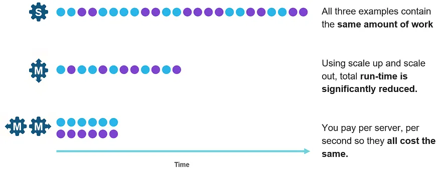
Although the amount of work is the same, using scale-up or scale-out, total run-time is significantly reduced. Since customers pay per-VM on a per-second basis, the cost is the same.
The following query lists warehouses and times that could benefit from multi-cluster warehouses based on the amount of queuing.
- LIST OF WAREHOUSES AND DAYS WHERE MCW COULD HAVE HELPED
 SELECT TO_DATE(START_TIME) as DATE
 ,WAREHOUSE_NAME
 ,SUM(AVG_RUNNING) AS SUM_RUNNING
 ,SUM(AVG_QUEUED_LOAD) AS SUM_QUEUED
 FROM "SNOWFLAKE"."ACCOUNT_USAGE"."WAREHOUSE_LOAD_HISTORY"
 WHERE TO_DATE(START_TIME) >= DATEADD(month,-1,CURRENT_TIMESTAMP())
 GROUP BY 1,2
 HAVING SUM(AVG_QUEUED_LOAD) >0
 ;
Elasticity of virtual warehouses
Stateless scaling
Virtual Warehouses are stateless compute resources. They can be created, destroyed, or resized at any point in an on-demand manner with no effect on the state of the data. By default, Virtual Warehouses are automatically provisioned when idle if a job is issued. Similarly, by default, the resources associated with a Virtual Warehouse are automatically released when there are no pending jobs. This elasticity allows customers to dynamically match compute resources to usage demands, independent of data volume.
When a job is submitted, each VM in the respective Virtual Warehouse cluster spawns a new process that lives only for the duration of its job. Any failures of these processes are quickly resolved by automatic retries.
Each user can have multiple Virtual Warehouses running at any given time, and each Virtual Warehouse may be running multiple concurrent jobs. Every Virtual Warehouse has access to the same shared tables, without the need to maintain its own copy of the data. Since virtual warehouses are private compute resources that operate on shared data, interference of different workloads from different organizational units is avoided. This makes it possible to have several Virtual Warehouses for jobs from different organizational units, often running continuously.
Multi-cluster autoscaling
To help control the usage footprint of auto-scaling multi-cluster warehouses, scaling policy options (economy, standard) can be used to control the relative rate at which clusters automatically start or shut down.
The Standard policy is the default and minimizes queuing by favoring starting additional clusters over conserving credits. With the standard policy, the first cluster starts immediately when either a query is queued or the system detects that there’s one more query than the currently running clusters can execute. Each successive cluster waits to start 20 seconds after the prior one has started. For example, if a warehouse is configured with 10 max clusters, it can take ~200 seconds to start all 10 clusters. Clusters shut down after 2 to 3 consecutive successful checks (performed at 1-minute intervals), which determine whether the load on the least-loaded cluster could be redistributed to the other clusters without spinning up the cluster again.
The Economy policy conserves credits by favoring keeping running clusters fully loaded rather than starting additional clusters, which may result in queries being queued and taking longer to complete. With the economy policy, a new cluster is started only if the system estimates there’s enough query load to keep the cluster busy for at least 6 minutes. Clusters shut down after 5 to 6 consecutive successful checks (performed at 1 minute intervals), which determine whether the load on the least-loaded cluster could be redistributed to the other clusters without spinning up the cluster again.
Scale-to-zero
A warehouse can be set to automatically resume or suspend, based on activity to only consume resources based on actual usage. By default, Snowflake automatically suspends the warehouse if it is inactive for a specified period of time. Also, by default, Snowflake automatically resumes the warehouse when any job arrives at the warehouse. Auto-suspend and auto-resume behaviors apply to the entire warehouse and not to the individual clusters in the warehouse.
Managing auto-suspend duration
We recommend setting the auto-suspend duration based on the ability of the workload to take advantage of caching at the ephemeral storage layer detailed earlier. This exercise involves finding the sweet spot for cost efficiency by balancing across the benefits of compute cost savings by suspending compute quickly and the price-performance benefits of Snowflake’s sophisticated caching. In general, our high level directional guidance is as follows:
- For tasks, loading, and ETL/ELT use cases, immediate suspension of virtual warehouses is likely to be the optimal choice.
- For BI and SELECT use cases, query warehouses are likely to be cost-optimal with ~10 minutes for suspension to keep data caches warm for end users.
- For DevOps, DataOps, and Data Science use cases, warehouses are usually cost-optimal at ~5 minutes for suspension as a warm cache is not as important for ad-hoc & highly unique queries.
We recommend experimenting with these settings for stable workloads to achieve optimal price-performance.
The following query flags potential optimization opportunities by identifying virtual warehouses with an egregiously long duration for automatic suspension after a period of no activity on that warehouse.
SHOW WAREHOUSES
;
SELECT "name" AS WAREHOUSE_NAME
,"size" AS WAREHOUSE_SIZE
FROM TABLE(RESULT_SCAN(LAST_QUERY_ID()))
WHERE "auto_suspend" >= 3600 // 3600 seconds = 1 hour
;
The following statement timeouts provide additional controls around how long a query is able to run before canceling it. This can help ensure that any queries that get hung up for extended periods of time will not cause excessive consumption of credits and also prevent the virtual warehouse from being suspended. This parameter is set at the account level by default and can also be optionally set at both the warehouse and user levels.
SHOW PARAMETERS LIKE 'STATEMENT_TIMEOUT_IN_SECONDS' IN ACCOUNT;
SHOW PARAMETERS LIKE 'STATEMENT_TIMEOUT_IN_SECONDS' IN WAREHOUSE <warehouse-name>;
SHOW PARAMETERS LIKE 'STATEMENT_TIMEOUT_IN_SECONDS' IN USER <username>;
The following query aggregates the percentage of data scanned from the ephemeral storage layer (cache) across all queries broken out by warehouse. Warehouses running querying/reporting workloads with a low percentage of data returned from caches indicate optimization opportunities (because warehouses may be suspending too quickly).
SELECT WAREHOUSE_NAME
,COUNT(*) AS QUERY_COUNT
,SUM(BYTES_SCANNED) AS BYTES_SCANNED
,SUM(BYTES_SCANNED*PERCENTAGE_SCANNED_FROM_CACHE) AS BYTES_SCANNED_FROM_CACHE
,SUM(BYTES_SCANNED*PERCENTAGE_SCANNED_FROM_CACHE) / SUM(BYTES_SCANNED) AS PERCENT_SCANNED_FROM_CACHE
FROM "SNOWFLAKE"."ACCOUNT_USAGE"."QUERY_HISTORY"
WHERE START_TIME >= dateadd(month,-1,current_timestamp())
AND BYTES_SCANNED > 0
GROUP BY 1
ORDER BY 5
;
“Warm pools” of running VMs to realize an “instant-on” experience
Virtual Machines (VMs) provide the requisite multi-tenant security and resource isolation — this is detailed in a subsequent section. However, since VMs are slow to start up (order of tens of seconds), cold starting them is not conducive to realize an instant-on experience. To work around this limitation, we use free pools of pre-started running VMs to sidestep the slow VM launch times and ameliorate any possible capacity challenges issues in (usually smaller) cloud regions lacking liquidity of VMs used by Snowflake.
Snowflake teams are bound by a demanding internal Service Level Objective (SLO) on lifecycle operations (such as start, stop, resume, suspend, scaling, etc.) to ensure an instant-on experience for customers. Aberrations from the SLO trigger on-call incident management workflows, post-incident analyses, and action items that are prioritized.
When user requests come in, running VMs in the free pool can be immediately assigned to virtual warehouses. However, to ensure efficient utilization of running VMs, accurate estimation of demand to size free pools optimally is important.
A predictive mechanism is used to size free pools which accounts for baseline demand as well as spikes that usually occur at the top-of-the-hour. Predictions are based on the historical demand for the same time slot in previous weeks while also accounting for prefetch duration to ensure timely VM provisioning and filtering of outliers due to one-off events to protect against over/under provisioning of free pool capacity.
Query Acceleration Service for on-demand bursts
Query Acceleration Service (QAS) enables another form of vertical scaling. It automatically adds compute capacity from the pool of running VMs for warehouses on an on-demand basis to offload & accelerate SQL queries . QAS is particularly useful for large table scans and/or handling bursty workload patterns.
When Snowflake detects a massive query that will scan gigabytes of data, the use of query acceleration can free up resources on the virtual warehouse cluster to execute other short-running queries from other users and is usually less expensive than scaling up to a larger warehouse and leads to more efficient use of resources. Effectively, the Query Acceleration Service acts like a powerful additional cluster that is temporarily available to deploy alongside existing virtual warehouses and when needed.
QAS compute resources billed per second. The SYSTEM$ESTIMATE_QUERY_ACCELERATION function and QUERY_ACCELERATION_ELIGIBLE View help identify queries that might benefit from QAS.
The following query identifies the queries that might benefit the most from the service by the amount of query execution time that is eligible for acceleration:
SELECT query_id, eligible_query_acceleration_time
FROM SNOWFLAKE.ACCOUNT_USAGE.QUERY_ACCELERATION_ELIGIBLE
ORDER BY eligible_query_acceleration_time DESC;
The following query identifies the queries that might benefit the most from the service in a specific warehouse mywh:
SELECT query_id, eligible_query_acceleration_time
FROM SNOWFLAKE.ACCOUNT_USAGE.QUERY_ACCELERATION_ELIGIBLE
WHERE warehouse_name = 'mywh'
ORDER BY eligible_query_acceleration_time DESC;
The following query identifies the warehouses with the most queries eligible in a given period of time for the query acceleration service:
SELECT warehouse_name, COUNT(query_id) AS num_eligible_queries
FROM SNOWFLAKE.ACCOUNT_USAGE.QUERY_ACCELERATION_ELIGIBLE
WHERE start_time > 'Mon, 29 May 2023 00:00:00'::timestamp
AND end_time < 'Tue, 30 May 2023 00:00:00'::timestamp
GROUP BY warehouse_name
ORDER BY num_eligible_queries DESC;
The following query identifies the warehouses with the most eligible time for the query acceleration service:
SELECT warehouse_name, SUM(eligible_query_acceleration_time) AS total_eligible_time
FROM SNOWFLAKE.ACCOUNT_USAGE.QUERY_ACCELERATION_ELIGIBLE
GROUP BY warehouse_name
ORDER BY total_eligible_time DESC;
Query Acceleration scale factor sets an upper bound on the amount of compute resources a warehouse can lease for acceleration. The scale factor is a multiplier based on warehouse size and cost. For example, if the scale factor is 5 for a Medium-sized warehouse (4 credits/hour), the warehouse can lease compute up to 5 times its size (i.e., 4 x 5 = 20 credits/hour). By default, the scale factor is set to 8 when Query Acceleration Service is used.
The following query identifies the upper limit for scale factor for a given warehouse with QAS enabled:
SELECT MAX(upper_limit_scale_factor)
FROM SNOWFLAKE.ACCOUNT_USAGE.QUERY_ACCELERATION_ELIGIBLE
WHERE warehouse_name = 'mywh';
The following query identifies the distribution of scale factors for a given warehouse with QAS enabled:
SELECT upper_limit_scale_factor, COUNT(upper_limit_scale_factor)
FROM SNOWFLAKE.ACCOUNT_USAGE.QUERY_ACCELERATION_ELIGIBLE
WHERE warehouse_name = '<warehouse_name>'
GROUP BY 1 ORDER BY 1;
Job scheduling in Virtual Warehouses
After compilation in the Snowflake Cloud Services layer, jobs are scheduled for execution by the Warehouse Scheduling Service (WSS) which tracks and throttles load on the warehouse with the aim of striking a balance between maximizing throughput and minimizing latency, maximizing utilization of warehouse clusters, and deterministic performance under contention.
WSS tracks memory and CPU usage across all the VMs of each Virtual Warehouse cluster. The memory capacity of a cluster is the available memory on each VM (after subtracting the footprint of OS and other system software) multiplied by the number of VMs. When main memory is exhausted during execution, Snowflake allows data to “spill” to disk. If memory pressure is excessive, jobs may get killed and retired.
CPU usage is a proxy for tracking concurrency. Each job runs with a Degree Of Parallelism (DOP) which is the number of processes executing the job simultaneously. The maximum DOP for a job is the number of processes per VM (upper bounded by the number of CPU cores on each VM) multiplied by the number of VMs available to execute the job (limited by the warehouse size selected by the customer). As an example, a warehouse with 4 VMs each with 8 vCPUs, has 8*4 = 32 DOP available, which means it can simultaneously run up to 32 jobs (for a singular concurrency workload) with a DOP of 1 simultaneously or 8 jobs (also for a singular concurrency workload) with a DOP of 4. Other combinations are possible, as long as the total DOP across all running jobs does not exceed 32. Based on the value of MAX_CONCURRENCY set by the cusotmer, the effective number of jobs that can be simultaneously run would be MAX_CONCURRENCY * MAX_DOP.
The Cloud Services layer receives jobs to schedule on available warehouse clusters and creates a “scheduling request” with WSS containing the required memory and requested DOP, which is estimated during compilation. WSS maintains a queue of other jobs waiting to run on available warehouse clusters. WSS decides whether the job is allowed to run or whether it has to wait in the queue. Eventually, WSS chooses a cluster of the warehouse for the job to run and informs the Cloud Services layer which sends the job to the chosen warehouse cluster for execution.
When jobs arrive at WSS, they are moved into a queue with FIFO behavior. If a job fails during execution and is rescheduled, it keeps its place in the queue and does not have to join at the back of the line. WSS iterates over jobs in the queue starting at the front and checks whether it is allowed to run on an available cluster based on availability of free memory and concurrency. If there are multiple eligible clusters, the job is scheduled on the one with the lowest current concurrency level. If no cluster is eligible, the job continues to wait in the queue. WSS makes a simplifying assumption that load will be evenly distributed across all VMs of the cluster.
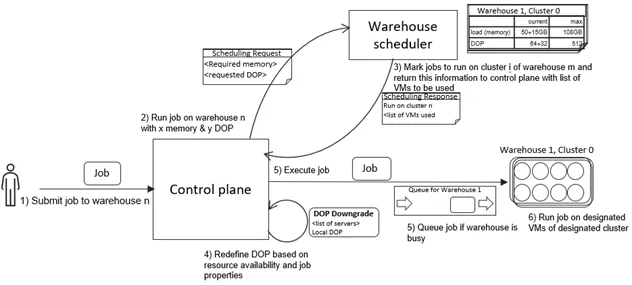
When WSS schedules jobs on the cluster, it increases the tracked resource balance of the cluster. The “scheduling response” contains the cluster chosen by WSS for the job and a list of all available VMs on that cluster. Based on this response, the Cloud Services layer (represented as “control plane” in the image above) may perform a “DOP Downgrade” and determine the VMs used to execute it. The downgraded DOP may also be larger or smaller than the requested DOP.
Once the DOP Downgrade has been completed, the job is sent to the Virtual Warehouse cluster for execution. After the execution has been completed, WSS frees the allocated resources.
WSS performs all scheduling and associated operations in memory to achieve high throughput and low latency. If a WSS node crashes, state is recovered by aggregating replicated state information from other nodes in the cluster.
Controls to inform concurrency levels
Since jobs running concurrently in a virtual warehouse share available resources, each incremental job gets a smaller share of resources. The MAX_CONCURRENCY_LEVEL parameter, which is set to 8 by default limits the number of concurrent queries running in a virtual warehouse.
Lowering the concurrency level can boost performance for individual jobs (especially if the jobs are complex or multi-statement queries) since each job gets a greater share of resources. However, lowering the concurrency level can cause increased job queuing. Other strategies such as using a dedicated virtual warehouse or using the Query Acceleration Service can boost the performance of a large or complex query without impacting the rest of the workload.
Furthermore, the STATEMENT_QUEUED_TIMEOUT_IN_SECONDS parameter can be used to cancel queries based on a timeout rather than let them remain in the queue for extended periods of time. This parameter can be set within the session hierarchy or at the warehouse level; when it is set for both a warehouse and a session, the lowest non-zero value is enforced. Its value is set to 0 by default (i.e., no timeout).
Similarly, the STATEMENT_TIMEOUT_IN_SECONDS parameter specifies the amount of time, in seconds, after which a running job (SQL query, DDL/DML statement, etc.) is canceled by the system. By default, it is set to 172800 seconds (i.e., 2 days).
Resource monitors & usage limits
Resource Monitors in virtual warehouses provide a mechanism to set up alerting and hard limits to prevent overspend via credit quotas for individual virtual warehouses during a specific time interval or date range. When warehouses reach a limit a notification and/or suspension can be initiated. Resource monitors can also be set up on a schedule to track and control credit usage by virtual warehouses.
To help control costs and avoid unexpected usage, we recommend using resource monitors, which consist of limits for a specified frequency interval and a set of warehouses to monitor. When limits are reached and/or are approaching, the resource monitor can trigger various actions, such as sending alert notifications and/or suspending warehouses.
The following query identifies all warehouses without resource monitors which have a greater risk of unintentionally consuming more credits than typically expected.
SHOW WAREHOUSES
;
SELECT "name" AS WAREHOUSE_NAME
,"size" AS WAREHOUSE_SIZE
FROM TABLE(RESULT_SCAN(LAST_QUERY_ID()))
WHERE "resource_monitor" = 'null'
;
Warehouse load and capacity sizing
Metrics exposed by Snowflake such can inform and guide optimizations to “right size” compute capacity.
Warehouse job load metrics measure the average number of jobs that were running or queued within a specific interval. It is computed by dividing the execution time (in seconds) of all jobs in an interval by the total time (in seconds) for the interval. A job load chart shows current and historical usage patterns along with total job load in intervals of 5 minutes to 1 hour (depending on the range selected) and individual load for each job status that occurred within the interval (Running, Queued).
Warehouse utilization metrics (in private preview) shows the utilization of resources as a percentage at a per-cluster and per-warehouse levels.

Warehouse load and utilization metrics can be used in conjunction to inform capacity allocation decisions. Some high-level postulates include:
If a workload has adequate throughput and/or latency performance AND (queued query load is low OR total query load <1 for prolonged periods) AND utilization is low (e.g., less than 50%):
- Consider downsizing the warehouse or reducing the number of clusters. Additionally, consider starting a separate warehouse and moving queued jobs to that warehouse
If a workload is running slower than desired (based on throughput and/or latency measurements) AND running query load is low AND utilization is high (e.g., greater than 75%):
- Consider upsizing the warehouse or adding clusters
If there are recurring usage spikes (based on warehouse utilization history):
- Consider moving queries that represent the spikes to a new warehouse or adding clusters. Also, consider running the remaining workload on a smaller warehouse
If a workload has considerably higher than normal load:
- Investigate which jobs are contributing to the higher load.
If the warehouse runs during recurring time periods, but the total job load is < 1 for substantial periods of time:
- Consider decreasing the warehouse size and/or reduce the number of clusters.
Storage and caching in Virtual Warehouses
Storage architecture
In addition to metadata (such as object catalogs, mappings from database tables to corresponding files in persistent storage, statistics, transaction logs, locks, etc.), two forms of state are used in Snowflake:
1/ Persistent storage of tables
Since tables are long-lived and may be read by many queries concurrently, persistent storage for tables requires strong durability and availability guarantees.
Remote, disaggregated, persistent storage such as Amazon S3 (or equivalent) is used because of its elasticity, high availability, and durability, despite relatively modest latency and throughput. Object storage solutions on cloud providers (such as Amazon S3 or equivalent) support storing immutable files, because of which they can only be overwritten in full. Snowflake takes advantage of cloud object storage support for reading parts of a file by partitioning tables horizontally into large, immutable files. Within each file, the values of each individual attribute or column are grouped together and compressed. Each file has a header that stores the offset of each column within the file, enabling the use of cloud object storage’s partial read functionality to only read columns needed for query execution.
2/ Intermediate data generated by query operators (e.g., joins) and consumed during executing queries
Since intermediate data is short-lived, low-latency & high-throughput access to prevent execution slowdown is preferred over strong durability guarantees. The SSD and main memory on virtual warehouse VMs provide ephemeral storage with the requisite latency and throughput performance needed for job execution; this is cleared when a virtual warehouse is suspended or stopped. This ephemeral storage layer is a write-through “cache” for persistent data to keep cached persistent files consistent and reduce the network load caused by compute-storage disaggregation.
Each virtual warehouse cluster has its own independent distributed ephemeral storage, which is used only by queries it runs. All virtual warehouses in the same account have access to the same shared tables via the remote persistent store and do not need to copy data from one virtual warehouse to another.
Spilling as a means to simplify memory management
When execution artifacts perform write operations of intermediate data, first, main memory on the same VM is used; if this memory is full, data is “spilled” to local disk/SSD; when local disk is full, data spills to remote persistent storage (object storage such as Amazon S3). This scheme removes the need to handle out-of-memory or out-of-disk errors.
Caching strategy
When the demands of intermediate data are low, the ephemeral storage layer is also used to cache frequently accessed persistent data files (as a lesser priority) using a “lazy” consistent hashing over file names and an LRU eviction policy. Each file is cached only on the virtual warehouse VM to which it consistently hashes within the cluster. This scheme enables locality without reshuffling cached data (which can interfere with ongoing jobs) when VMs are added/removed to virtual warehouse clusters during resize or scaling operations — achieved by using the copy of data remote persistent storage, which also ensures eventual consistency of data in the ephemeral storage layer.
Since each persistent storage file is cached on a specific VM (for a fixed virtual warehouse size), operations on a persistent storage file are scheduled to the VM on which its file consistently hashes to. Since jobs are scheduled for cache locality, job parallelism is tightly coupled with the consistent hashing of files.
To avoid imbalanced partitions and overloading of a few virtual warehouse VMs due to hashing based on file names, work is load-balanced across VMs in the same cluster based on whether the expected completion time of an execution artifact is lower on a different VM. When execution artifacts are moved, files needed to execute the operation are read from persistent storage to avoid increasing load on already overloaded straggler VMs where the execution was initially scheduled. This also helps when some VMs may be executing much slower than others (due to a number of factors including cloud provider virtualization issues, network contention, etc.).
Snowflake’s scheduling logic attempts to find a balance between co-locating execution artifacts with cached persistent storage versus placing all execution artifacts on fewer virtual warehouse VMs. While the former minimizes network traffic for reading persistent data, it comes with the risk of increased network traffic for intermediate data exchange since jobs may be scheduled on all VMs of the virtual warehouse cluster. The latter obviates the need for network transfers for intermediate data exchange but can increase network traffic for persistent storage reads.
Real-world data has shown that the amount of data written to ephemeral storage is in the same order of magnitude as the amount of data written to remote persistent storage. Despite the size of ephemeral storage capacity being significantly lower (~0.1% on average) than the size of persistent storage, our data shows that Snowflake’s caching scheme enables average cache hit rates of ~80% for read-only queries and ~60% for read-write queries.
Security and resource isolation for multi-tenancy
Snowflake provides a well-thought-out and multi-layered security model to achieve defense in depth. All artifacts in object storage use per-object encryption. The security model for virtual warehouses is designed to protect against cross-account information disclosure and cross-job information disclosure within the same customer account. Virtual Machine isolation provides the basis for multi-tenant isolations across Snowflake accounts. Furthermore, sandboxes inside VMs with Linux kernel primitives similar to Docker Containers such as cgroups, kernel namespaces, secomp protect against cross-job information disclosure within the same customer account.
Virtual Machines (VMs) provide the requisite multi-tenant security and resource isolation since each VM runs in an isolated environment with its own virtual hardware, page tables, and kernel.
At Snowflake, we’ve determined that traditional shared kernel container isolation (using primitives such as cgroups, secomp, and kernel namespaces) alone in the absence of VM isolation doesn’t suffice our bar for multi-tenancy. Although containers start rapidly, the large kernel system call surface of the shared kernel present challenges based on the track record of CVEs that are found & fixed compared to the hypercall interface used for VM isolation (since VMs come with its own virtual hardware, page tables, and kernel).
In Virtual Warehouses, VMs that comprise a Virtual Warehouse are private computing resources are are dedicated solely to that Virtual Warehouse; they aren’t shared across Virtual Warehouses. Additionally, Virtual Warehouses are also stateless compute resources. They can be created, destroyed, or resized at any point in an on-demand manner with no effect on the state of the data. This results in strong performance isolation for jobs since each customer job runs on exactly one Virtual Warehouse.
When a job is submitted, each VM in the respective Virtual Warehouse cluster spawns a new process that lives only for the duration of its job. Any failures of these processes are quickly resolved by automatic retries.
Each user can have multiple Virtual Warehouses running at any given time, and each Virtual Warehouse may be running multiple concurrent jobs.
Network security
Virtual Warehouse VMs require external network access for: 1/ Communication with the Cloud Services layer 2/ To share data during job execution with other warehouse VMs, 2/Access to Local Cloud Storage, 3/Access to Remote Cloud Storage, 4/ Access to API Gateway.
Snowflake treats all network traffic from warehouse clusters as untrusted. Traffic to internal services is limited to a set of authenticated endpoints. All traffic to external networks traverses an egress proxy that enforces access control policies, blocks access to unauthorized endpoints, and reports unexpected activity to Snowflake’s incident response team.
To protect against cross-account information disclosure, the Cloud Services layer validates all communication to be appropriate by verifying matching of the IP address on record for the VM/proxy/job in question. Requests from IPs internal to Snowflake are treated specially by the Cloud Services layer with explicit IP blocks for Virtual Warehouses. Additionally, in Virtual Warehouse peer-to-peer communication, all participating VMs include a signature signed by a shared secret which is validated to confirm membership in the current warehouse. Furthermore, rate limiting prevents Virtual Warehouse VMs from launching a DoS attack against the Cloud Services layer.
Furthermore, flow logging of virtual network traffic flow captures metrics for all source/destination IPs pairs is used to identify expected network paths, connection rates along those paths, and alerts for when traffic violates established baselines. This will, for example, allow the identification of Warehouse VMs sending data to unexpected destinations and then quarantine that VM for forensic inspection.
Security isolation for customer code in Python/Scala/Java
Unlike SQL which comes with a limited language surface, code in Java/Python/Scala for User Defined Functions (UDF) and Stored procedures presents a larger security attack surface.
This code is run on the same virtual warehouse VMs that execute the rest of the job for performance reasons. In addition to the use of VMs (that aren’t reused across accounts) for multi-tenant compute isolation, a secure sandbox using Linux kernel primitives such as cgroups, namespaces, secomp, eBPF, chroot prevents code from accessing information outside of its environment (scoped to the current job) or affecting the operation of other parts of Snowflake; other virtual warehouse resources such as its network and namespaces are also isolated from the contents of the sandbox.
Each Java/Python/Scala job gets a new sandbox and includes “just enough” read-only software needed to run code while a chroot directory tree is used for a few required writable directories and a temporary one that provides scratch space. JAR Java packages, Python packages, and data files are shared via a read-only bind-mount directory. The sandbox is run in a cgroup to limit the executing code’s memory, CPU, and PID usage. Spawning threads is supported to enable multi-processor use cases. Furthermore, additional lockdown is provided via restrictions around network access through explicit allow-listing (via IPC namespaces & eBPF to prevent non-allow-listed artifacts from opening of UNIX sockets connecting to processes outside the sandbox), filesystem isolation (via the use of mount namespace and chroot to minimal read-only filesystem), blocking visibility into other processes on the VM (via a new process namespace), and blocking unneeded kernel APIs using seccomp (e.g., forking child processes or exec-ing executables). ptrace is used to govern system calls for threat detection.
After job completion, environment variables on the VM are cleared, open sockets are closed, all VM credentials are removed, and local caches, temporary files, logs are cleared. As an additional defense-in-depth measure, a monitor process sends a kill signal to the process running customer code if it doesn’t exit within expected time bounds.
To further protect against the hypothetical risk of escaping the sandbox and an attacker leaving a persistent process or rootkit on Virtual Warehouse VMs, VMs that have run Python/Java customer code are marked as “not for reuse”. Virtual warehouse scheduling and free pool management mechanisms ensure that such VMs are not assigned to a different account/customer as a defense-in-depth mechanism to prevent cross-account information disclosure risks. When such VMs are released, they go into a dedicated per-account free pool. When allocating new VMs, they are first pulled from per-account free pools. Additionally, VMs in the per-account free pools are periodically terminated.
Even if there is a hypothetical sandbox breakout if a large number of zero-day kernel exploits are used sequentially, additional defense-in-depth mechanisms are designed to contain the breakout. First, the exploit is contained in a VM running in the customer’s account. This VM is isolated from Snowflake services and VMs in Snowflake’s local network using cloud networking security groups applied to its network-virtualized “Virtual Private Cloud”. Furthermore, since credentials in possession by the attacker from such a hypothetical breakout are scoped for the specific account and specific VM, customer data isn’t accessible.
Managing software updates
Snowflake’s code rollout to virtual warehouses workflows ensures fast delivery of new features, security updates, and improved service to customers. The process is fully automated to avoid manual errors. Snowflake’s release process includes multiple layers of testing, including unit testing, regression testing, integration testing, performance and load testing at scale on pre-production and production-like environments.
Virtual Warehouse upgrades are orchestrated safely and wait until running jobs complete. Based on the nature of the upgrade, different strategies are followed. The Cloud Services layer’s topology and traffic routing features are used to route new jobs to the new VMs.
When VMs are added to the free pool, they are started with the latest patched and up-to-date VM images. As a part of the process to attach VMs from the free pool to virtual warehouses clusters after lifecycle operations such as start or resume, the latest binaries are downloaded and installed to keep software in warehouse VMs patched and up-to-date. This process is performed in a latency-critical manner to ensure that the “instant-on” properties for lifecycle operations aren’t impacted.
For major changes such as changes to VM SKU/size or OS major version, both the old and new (upgraded) variants of the virtual warehouse are concurrently kept running; the old version continues to run existing jobs, while new jobs are routed to the new (upgraded) variant. Finally, the old version of the virtual warehouse is discarded after running jobs complete. The state is caches across both versions of the same warehouse are proactively managed to mitigate performance impacts from cache misses during such migrations — where jobs of the workloads are split across old and new versions of the same virtual warehouses.
Similarly, updates can be rolled back. While a high bar for testing is maintained, some bugs may only be seen in production.
We run two copies of binaries concurrently for each cloud region Snowflake operates in — the old (likely more stable) and new version; the old version kept idle and not actively serving traffic.
In case of any major issues related to software updates that impacts a large number of customers, we perform an instantaneous rollbacks at the granularity of a cloud region by routing new requests to the old, stable software version.
Additionally, we also perform per-customer targeted rollback based on the blast radius of issues. Not all bugs hit customers equally, as many customers have unique workloads. For example, a bug may in a software update may only affect a small subset of customers if their particular workloads exercise specific code paths. In such cases it is unnecessary to do full rollbacks for all customers and we resort to per-customer rollbacks by explicitly mapping only affected accounts to the old (more stable) software version.
Health management and self-healing
At scale, not all VMs under management will be healthy and functional. To mitigate this, automation monitors the health of each VM on each cluster in each virtual warehouse. A warehouse VM is deemed healthy if it has a heartbeat to the Cloud Services layer within a pre-specified time interval and can respond to an on-demand health check within another pre-specified time interval.
A health check is sent to warehouse VMs when system conditions such as kernel warnings, network connectivity issues, internal exceptions, etc. indicate that it is no longer healthy. This causes the warehouse VM to checksum certain binaries, check for kernel errors and connectivity with other VMs in the same cluster. After these checks have completed, results are sent back to the Cloud Services layer. VMs that fail their health checks or heartbeats are replaced with healthy ones from the warm pool of running VMs. The replaced VMs are marked as “failed”, precluded from running new jobs, and returned to the cloud provider; the health indicators of such VMs are also logged to enable later analysis.
Dealing with job failures with retires
Virtual warehouses are stateless compute resources. When a job is submitted, each VM in the respective Virtual Warehouse spawns a new process that lives only for the duration of its job and does not cause externally visible effects (even if it is a part of an update statement), because table files are immutable. Any failures of these processes are thus contained and quickly and easily resolved by automatic retries.
Future capabilities
Today, customers need to translate the criteria they reason about such as workload (as a collection of queries), desired completion time for the workload (a.k.a Service Level Objective), and cost budget into appropriate knob settings for compute capacity (via settings for warehouse size, warehouse type, cluster counts, scaling policy, etc.). We’re aiming to reduce/remove the overhead of capacity sizing and enable customers to provide inputs that map to the criteria they reason about such as workload (as a collection of jobs), cost budget, and SLO.
Furthermore, we’re looking in invest in stronger sandbox isolation mechanisms via the use of technologies such as microVMs (e.g., Firecracker, Kata Containers, etc.) or offloading a subset of syscall execution to userspace (e.g., gVisor) to unlock additional use cases with custom code in Python/Java that are constrainer with the current sandbox including support for OCI containers.
Conclusion
This post details the design, architecture, and operation of Snowflake’s fully-managed serverless data plane with scale-to-zero properties including: 1/ how Virtual Warehouses host and run customer jobs by handling elasticity, scalability, scheduling, utilization, and availability behind the scenes, 2/ the mechanisms used to provide both multi-tenant security isolation without compromising an “instant-on” experience.
