Improve Snowflake price-performance by optimizing storage

This blog post discusses strategies and best practices to improve Snowflake price-performance by reducing compute spend via the use of built-in mechanisms to store similar data together, create optimized data structures, and/or define specialized data sets.

Snowflake storage — a primer

When a table’s storage is partitioned, queries run faster when unneeded partitions are skipped (a.k.a pruning). Snowflake tables are automatically organized into micro-partitions via range-partitioning on every column, with a maximum size of ~16MiB when compressed (~120 MiB uncompressed). If a query filters, joins, or aggregates along the dimensions used for partitioning, fewer micro-partitions are scanned to return results.

Once created, a micro-partition is immutable. The partition-key columns are not specified as every column has maximum and minimum values in the metadata. As a result, every column in the table can potentially be used to determine if a micro-partition can be pruned.

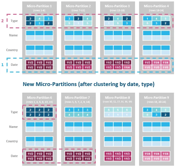
Automatic Clustering

Automatic Clustering helps reorganize table data to align with query patterns to process only the relevant data from large tables, speeding up queries to help consume fewer compute credits.

You can set a cluster key to change the organization of micro-partitions so that data is clustered around specific dimensions (i.e., columns). This can help improve the performance of queries that filter, join, or aggregate by the columns defined in the cluster key.

Once enabled, Automatic Clustering updates micro-partitions as new data is added to the table. The pricing for auto clustering is based on credits for background clustering maintenance.

Automatic clustering is performed in an incremental and non-blocking manner in the background without hindering running workloads.

Automatic Clustering can benefit cases where many queries perform filter/join/aggregate operations on the same few columns, as well as range queries with large table scans or queries with an inequality filter. We recommend picking the most important queries based on frequency and latency requirements and a clustering key that maximizes the performance of those queries. Usually, the largest price-performance boost comes from a WHERE clause that filters on a column of the cluster key. For example, the following query executes with superior price-performance if the shipdate column is the table’s cluster key because the WHERE clause scans a large amount of data.

SELECT
 SUM(quantity) AS sum_qty,
 SUM(extendedprice) AS sum_base_price,
 AVG(quantity) AS avg_qty,
 AVG(extendedprice) AS avg_price,
 COUNT(*) AS count_order
 FROM lineitem
 WHERE shipdate >= DATEADD(day, -90, to_date('2023–01–01));

The following query shows the average daily credits consumed by Auto Clustering grouped by week over the last year. It can help identify anomalies in daily averages over the year and help investigate any unexpected changes in consumption.

WITH CREDITS_BY_DAY AS (
SELECT TO_DATE(START_TIME) as DATE
,SUM(CREDITS_USED) as CREDITS_USED
FROM "SNOWFLAKE"."ACCOUNT_USAGE"."AUTOMATIC_CLUSTERING_HISTORY"
WHERE START_TIME >= dateadd(year,-1,current_timestamp()) 
GROUP BY 1
ORDER BY 2 DESC 
 )
 
SELECT DATE_TRUNC('week',DATE)
,AVG(CREDITS_USED) as AVG_DAILY_CREDITS
FROM CREDITS_BY_DAY
GROUP BY 1
ORDER BY 1
;

The following query shows the automatic clustering history for the past week for a specified table in the current account:

select *
 from table(information_schema.automatic_clustering_history(
 date_range_start=>dateadd(d, -7, current_date),
 date_range_end=>current_date,
 table_name=>'mydb.myschema.mytable'));

Materialized Views

Materialized Views store frequently used projections and aggregations to avoid expensive re-computations, resulting in superior price-performance. The results from Materialized Views are guaranteed to be up-to-date via asynchronous and incremental maintenance. The pricing is based on refreshes and additional storage.

A materialized view is a pre-computed data set derived from a query specification and stored for later use. Querying a materialized view is faster than executing a query against the base table of the view.

Behind the scenes, a materialized view is effectively a pre-computed data set derived from a SELECT statement that is stored for later use. Because data is pre-computed, querying a materialized view is faster than executing a query against the base table on which the view is defined. A materialized view cannot be based on more than one table.

Materialized views are recommended for workloads composed of common, repeated query patterns that return a small number of rows and/or columns relative to the base table. We recommend using it in a focused manner on specific query/subquery calculations that are both intensive and frequent — e.g., aggregation and analysis on a small subset of semi-structured data.

The following query shows the average daily credits consumed by Materialized Views grouped by week over the last year. It can help identify anomalies in daily averages over the year, which provides launching points to investigate unexpected changes in consumption.

WITH CREDITS_BY_DAY AS (
SELECT TO_DATE(START_TIME) as DATE
,SUM(CREDITS_USED) as CREDITS_USED
FROM "SNOWFLAKE"."ACCOUNT_USAGE"."MATERIALIZED_VIEW_REFRESH_HISTORY"
WHERE START_TIME >= dateadd(year,-1,current_timestamp()) 
GROUP BY 1
ORDER BY 2 DESC 
 )
 
SELECT DATE_TRUNC('week',DATE)
,AVG(CREDITS_USED) as AVG_DAILY_CREDITS
FROM CREDITS_BY_DAY
GROUP BY 1
ORDER BY 1
;

The following query provides a full list of materialized views and the volume of credits consumed via the service over the last 30 days, broken out by day. Any irregularities in the credit consumption or consistently high consumption are flags for additional investigation.

SELECT
TO_DATE(START_TIME) as DATE
,DATABASE_NAME
,SCHEMA_NAME
,TABLE_NAME
,SUM(CREDITS_USED) as CREDITS_USED
FROM "SNOWFLAKE"."ACCOUNT_USAGE"."MATERIALIZED_VIEW_REFRESH_HISTORY"
WHERE START_TIME >= dateadd(month,-1,current_timestamp()) 
GROUP BY 1,2,3,4
ORDER BY 5 DESC 
;

The following query shows the materialized view maintenance history for the past week for the current account:

select *
 from table(information_schema.materialized_view_refresh_history(
 date_range_start=>dateadd(d, -7, current_date),
 date_range_end=>current_date));

The following query shows the maintenance history for the past week for a specified materialized view in the current account:

select *
 from table(information_schema.materialized_view_refresh_history(
 date_range_start=>dateadd(d, -7, current_date),
 date_range_end=>current_date,
 materialized_view_name=>'mydb.myschema.my_materialized_view'));

Search Optimization Service

Search Optimization Service makes it possible to quickly find “needles in the haystack” to return a small number of rows from large tables using highly selective filters. This includes data exploration and filtering workloads such as investigative log searches and threat/anomaly detection. It accelerates point lookup queries on all columns of supported types on large tables by building a persistent data structure that is optimized for a particular type of search.

In the example above, Search Optimization helps reduce the number of partitions to be scanned from 15 to 1, helping speed up a query to find all rows with a certain name.

You can enable the Search Optimization Service for an entire table or for specific columns. If the filters are sufficiently selective, equality searches, substring searches, and geo searches against those columns can be sped up significantly.

When specific queries access a well-defined subset of a table’s data, we recommend using the characteristics of the query to decide whether to use Search Optimization or Materialized Views. For example, the presence of important point lookup queries can inform the use of Search Optimization for a table or column.

You can run the SYSTEM$ESTIMATE_SEARCH_OPTIMIZATION_COSTS function to estimate the cost of adding Search Optimization to a column or entire table. The estimated costs are proportional to the number of columns that will be enabled and how much the table has recently changed.

In the example below, the following query executes faster with Search Optimization if the sender_ip column has a large number of distinct values.

SELECT error_message, receiver_ip
 FROM logs
 WHERE sender_ip IN ('198.2.2.1', '198.2.2.2');

The following query provides a full list of tables with search optimization and the volume of credits consumed via the service over the last 30 days, broken out by day. Any irregularities in the credit consumption or consistently high consumption are flags for additional investigation.

SELECT
TO_DATE(START_TIME) as DATE
,DATABASE_NAME
,SCHEMA_NAME
,TABLE_NAME
,SUM(CREDITS_USED) as CREDITS_USED
FROM "SNOWFLAKE"."ACCOUNT_USAGE"."SEARCH_OPTIMIZATION_HISTORY"
WHERE START_TIME >= dateadd(month,-1,current_timestamp()) 
GROUP BY 1,2,3,4
ORDER BY 5 DESC 
;

The following query shows the average daily credits consumed by Search Optimization grouped by week over the last year. It can help identify anomalies in daily averages over the year, which can help investigate unexpected changes in consumption.

WITH CREDITS_BY_DAY AS (
SELECT TO_DATE(START_TIME) as DATE
,SUM(CREDITS_USED) as CREDITS_USED
FROM "SNOWFLAKE"."ACCOUNT_USAGE"."SEARCH_OPTIMIZATION_HISTORY"
WHERE START_TIME >= dateadd(year,-1,current_timestamp()) 
GROUP BY 1
ORDER BY 2 DESC 
 )
 
SELECT DATE_TRUNC('week',DATE)
,AVG(CREDITS_USED) as AVG_DAILY_CREDITS
FROM CREDITS_BY_DAY
GROUP BY 1
ORDER BY 1
;

Cost considerations & concurrent use of multiple storage optimizations

Implementing storage strategies can require greater time and financial investments compared to other performance optimizations (such as re-writing individual queries, optimizing warehouse sizing, etc.), but can unlock meaningful price-performance improvements.

Snowflake uses compute resources to maintain storage optimizations as new data is added to a table. The more changes to a table, the higher the maintenance costs. If a table is constantly updated, the cost of maintaining a storage optimization increases.

Unlike Search Optimization and Materialized Views, Automatic Clustering reorganizes existing data rather than creating additional storage. Similar to DML operations, reclustering consumes credits depending on the size of the table and amount of data. Each time data is reclustered, rows are physically grouped based on the clustering key for the table, resulting in new micro-partitions. Adding a small number of rows to a table can cause all micro-partitions that contain those values to be recreated which can result in significant data turnover and increased storage cost because the original micro-partitions are retained to support Snowflake’s “Time Travel” and “Fail-safe” features.

The following query shows the cost of built-in storage optimization capabilities:

USE DATABASE SNOWFLAKE;
USE SCHEMA ACCOUNT_USAGE;
SET CREDIT_PRICE = 4.00; - edit this number to reflect credit price
SET TERM_LENGTH = 12; - integer value in months
SET TERM_START_DATE = '2023–01–01';
SET TERM_AMOUNT = 100000.00; - number(10,2) value in dollars
WITH CONTRACT_VALUES AS (
SELECT
 $CREDIT_PRICE::decimal(10,2) as CREDIT_PRICE
 ,$TERM_AMOUNT::decimal(38,0) as TOTAL_CONTRACT_VALUE
 ,$TERM_START_DATE::timestamp as CONTRACT_START_DATE
 ,DATEADD(month,$TERM_LENGTH,$TERM_START_DATE)::timestamp as CONTRACT_END_DATE
),
PROJECTED_USAGE AS (
SELECT
 CREDIT_PRICE
 ,TOTAL_CONTRACT_VALUE
 ,CONTRACT_START_DATE
 ,CONTRACT_END_DATE
 ,(TOTAL_CONTRACT_VALUE)
 /
 DATEDIFF(day,CONTRACT_START_DATE,CONTRACT_END_DATE) AS DOLLARS_PER_DAY
 , (TOTAL_CONTRACT_VALUE/CREDIT_PRICE)
 /
 DATEDIFF(day,CONTRACT_START_DATE,CONTRACT_END_DATE) AS CREDITS_PER_DAY
 FROM CONTRACT_VALUES
)

- COMPUTE FROM CLUSTERING
SELECT
 'Auto Clustering' AS WAREHOUSE_GROUP_NAME
 ,DATABASE_NAME || '.' || SCHEMA_NAME || '.' || TABLE_NAME AS WAREHOUSE_NAME
 ,NULL AS GROUP_CONTACT
 ,NULL AS GROUP_COST_CENTER
 ,NULL AS GROUP_COMMENT
 ,ACH.START_TIME
 ,ACH.END_TIME
 ,ACH.CREDITS_USED
 ,$CREDIT_PRICE
 ,($CREDIT_PRICE*ACH.CREDITS_USED) AS DOLLARS_USED
 ,'ACTUAL COMPUTE' AS MEASURE_TYPE
from SNOWFLAKE.ACCOUNT_USAGE.AUTOMATIC_CLUSTERING_HISTORY ACH
UNION ALL

 - COMPUTE FROM MATERIALIZED VIEWS
SELECT
 'Materialized Views' AS WAREHOUSE_GROUP_NAME
 ,DATABASE_NAME || '.' || SCHEMA_NAME || '.' || TABLE_NAME AS WAREHOUSE_NAME
 ,NULL AS GROUP_CONTACT
 ,NULL AS GROUP_COST_CENTER
 ,NULL AS GROUP_COMMENT
 ,MVH.START_TIME
 ,MVH.END_TIME
 ,MVH.CREDITS_USED
 ,$CREDIT_PRICE
 ,($CREDIT_PRICE*MVH.CREDITS_USED) AS DOLLARS_USED
 ,'ACTUAL COMPUTE' AS MEASURE_TYPE
from SNOWFLAKE.ACCOUNT_USAGE.MATERIALIZED_VIEW_REFRESH_HISTORY MVH
UNION ALL

 - COMPUTE FROM SEARCH OPTIMIZATION
SELECT
 'Search Optimization' AS WAREHOUSE_GROUP_NAME
 ,DATABASE_NAME || '.' || SCHEMA_NAME || '.' || TABLE_NAME AS WAREHOUSE_NAME
 ,NULL AS GROUP_CONTACT
 ,NULL AS GROUP_COST_CENTER
 ,NULL AS GROUP_COMMENT
 ,SOH.START_TIME
 ,SOH.END_TIME
 ,SOH.CREDITS_USED
 ,$CREDIT_PRICE
 ,($CREDIT_PRICE*SOH.CREDITS_USED) AS DOLLARS_USED
 ,'ACTUAL COMPUTE' AS MEASURE_TYPE
from SNOWFLAKE.ACCOUNT_USAGE.SEARCH_OPTIMIZATION_HISTORY SOH
UNION ALL

You can implement more than one of these strategies for a table, and an individual query with multiple filters could potentially benefit from both Automatic Clustering and Search Optimization. If more than one strategy can potentially improve the price-performance of a query, we recommend starting with Automatic Clustering or Search Optimization because other queries with similar access patterns can also be improved.

Since there can be only one cluster key, if different queries against a table act upon different columns, we recommend using Search Optimization or a Materialized View. For queries that return more than a few records, we recommend using Automatic Clustering over Search Optimization (which is best suited for point lookup queries that return a small number of rows).

It is also noteworthy that the cost of maintaining Materialized Views or Search Optimization can be significant when Automatic Clustering is enabled for the underlying table because reclustering activities can trigger compute usage towards ongoing maintenance of Materialized Views and Search Optimization. Additionally, Search Optimization and Materialized Views incur the cost of additional storage and require Snowflake’s Enterprise Edition or higher, which increases the price of a credit.

Furthermore, Search Optimization and Query Acceleration can also be used together — after Search Optimization prunes micro-partitions not needed for a query, the rest of the work is accelerated.

Conclusion and recap

Different types of queries benefit from different storage strategies. You can experiment to discover which strategy best fits a workload. We recommend starting small and carefully tracking the initial & ongoing costs before committing to a more extensive implementation.