Super-charge Snowflake Query Performance with Micro-partitions

For all data storage systems, how data is written on disk or in memory has a large impact on the performance of querying that data. In traditional database systems, a primary index is used to group data by one or many fields for better query performance when using those fields. Rows sharing the same values in these fields are written to the same location or in close proximity for fast retrieval when a query uses the primary index fields. A secondary index can be used to point to rows matching a filtered set of predicates.

By default, Snowflake does not use a primary index but does provide features to add the equivalent of primary and secondary indexes to a table.

• Auto-clustering can give the same benefit as a primary index. Data is re-arranged after it is written to be clustered based on the fields chosen.
• Search optimisation service can be used to provide secondary index benefits.

Both of these features involve extra compute and cloud services costs to rewrite data. If you use them on a table that has an inefficient micro-partition profile, there is more movement of data and therefore more compute. More compute equals higher cost. From our experience it is better to focus on improving the micro-partitions profile of your tables first before using either feature. Once you gained as much efficiency as you can from improving the micro-partitions underneath your table, these features will be more efficient and cost-effective for it.

Micro-partitions

Snowflake stores all data in small units called micro-partitions. Snowflake provides a very good starter documentation on the feature here.

Micro-partitions & Data Clustering | Snowflake Documentation

In summary, micro-partitions are:

• Between 50 MB and 500 MB of uncompressed data.
• Groups of rows are mapped into individual micro-partitions, organized in a columnar fashion.
• Immutable, once written, cannot be updated. Updates to rows result in new micro-partitions being written.
• An individual micro-partition is unique to a table. They are not shared between tables.

Snowflake stores metadata about all rows stored in a micro-partition, such as:

• The range of values for each of the columns in the micro-partition.
• The number of distinct values.

Query execution

When a query is executed, Snowflake uses the micro-partition metadata to find which micro-partitions it needs to access to fulfil the query. Snowflake describes this as query pruning. By pruning the number of micro-partitions that need to be accessed, query time can be dramatically reduced.

Monitor clustering

Snowflake provides a good facility to monitor the clustering of micro-partitions in a table with the SYSTEM$CLUSTERING_INFORMATION system function.

SELECT SYSTEM$CLUSTERING_INFORMATION(‘table1’, ‘(col1)’);

To check how clustered a table is, you need to supply the table name and the name of column or columns you wish to check. The function will return a string in JSON format with several values. The most important of which are:

total_partition_count — the number of micro-partitions on the table.

average_overlaps — the average number of micro-partitions that have to be checked for the column values supplied. A higher number indicates that the table is not well-clustered.

average_depth — the average overlap depth of each micro-partition in the table. A high number indicates the table is not well-clustered.

Controlling micro-partitions

The best way to maintain efficient micro-partitions on a table is by being considerate with how you write and update records on the table. This can mean ordering the data on insert by the fields used to query. Snowflake will use this as an instruction or hint on how to generate micro-partitions. For example, if most of your queries contain a customer or account id, you could order your inserts by this column first. If it is time series data, it may be better to order by a date value. The trick is to order by the field that will be most commonly used in your queries. The fields you pick should have a low number of unique values, also known as low cardinality. If you choose a field that has a high number of unique values, you will end up with too many micro-partitions. For time series data, it may be better to order by the day part of the date, not the timestamp. Including an order by in the insert statement may add a small overhead on write time but better micro-partitions will result in a quicker read time.

If you have a high amount of updates, this can cause issues as when you update a record, Snowflake marks the older record as deleted and writes new micro-partitions for the updated records. You can’t use order by for update or merge statements. Therefore you may need to consider other approaches.

Insert Overwrite

For smaller tables, it may be enough to insert overwrite the table each time you update the table. This can be a quick operation and works well where you have more reads than writes. In this case, you will be looking to offset the increased cost of writes with the lower cost of reads.

Deferred merge

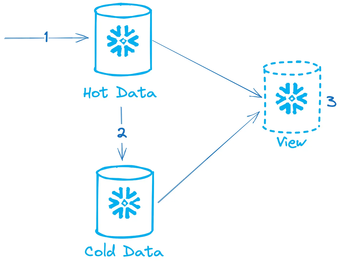
Deferred merge is a pattern whereby you maintain a temporary or hot data table (1) with changed or new records for an interval of time. When that time is up, you merge the temporary table into the main or cold data table (2) in one batch to ensure maintenance of micro-partitions. The hot data table is truncated at the time of merging into the cold data table. A view (3) can be written to provide a single interface to access all data.

Deferred merge can be a good option when you need to load data very often. Writing data frequently to a single table will mean the creation of lots of smaller inefficient micro-partitions. And as maintenance needs to be done at a table level, it can be expensive to fix this on a larger table retrospectively. Deferred merge works by writing new data into a temporary table until there are enough rows to create larger micro-partition in the main table. This ensures the main table maintains an efficient micro-partition profile. For append-only tables where records are only being inserted, not deleted or updated, deferred merge can be very simple. However where rows are being updated or deleted, you will need logic in the view to ignore the unchanged records in the cold data table.

There are many options on how you can implement a deferred merge pattern that deserve a blog post by itself.

Avoid using merge statement

If you have a mixed workload of inserts and updates, you may be tempred to use the Merge statement to reduce code written. However it does cause problems when trying to maintain a good micro-partition profile on a table. This is because you cannot use the order by statement for inserts performed via a merge statement. It may be better to split the merge into separate insert and update statements depending on your use case.

Maintenance jobs

Using the output from SYSTEM$CLUSTERING_INFORMATION, you could build a job that rebuilds a table based on the clustering information. You can put this sort of statement in a task that runs daily. You could make it smarter by adding a lookup table to control which tables are checked.

execute immediate
$$
declare
average_depth float;
begin
select parse_json(system$clustering_information(‘TABLE_1’, ‘(CLUSTERING_KEY_1)’)):total_partition_count::int as total_partition_count INTO :average_depth;
if (average_depth > 10) then
//insert overwrite into TABLE1 select * from TABLE_1 order by CLUSTERING_KEY_1;
return ‘Partition depth is ‘ || :average_depth || ‘. Ran insert overwrite.’;
else
return ‘Partition depth is ‘ || :average_depth || ‘. Did not run insert overwrite.’;
end if;
end;
$$;

Thanks to https://www.linkedin.com/in/greg-pavlik-9339091/ from Snowflake for providing this code example.

Examples

Using a real table that I have access to, we can check how much difference a good micro-partition profile can make to query performance.

Using the SYSTEM$CLUSTERING_INFORMATION function we can see the current profile of the table.

SELECT SYSTEM$CLUSTERING_INFORMATION(‘schema_name.table_name’,’(column_name)’);

{ “cluster_by_keys” : “LINEAR(column_name)”, “total_partition_count” : 10149, “total_constant_partition_count” : 20, “average_overlaps” : 10106.3529, “average_depth” : 10070.3322, “partition_depth_histogram” : { “00000” : 0, “00001” : 20, “00002” : 0, “00003” : 0, “00004” : 0, “00005” : 0, “00006” : 0, “00007” : 0, “00008” : 0, “00009” : 0, “00010” : 0, “00011” : 0, “00012” : 0, “00013” : 0, “00014” : 0, “00015” : 0, “00016” : 0, “08192” : 2, “16384” : 10127 }, “clustering_errors” : [ ] }

The main fields to look at here are “total_partition_count” : 10149 and “average_depth” : 10070.3322. This indicates that to query by the column_name specified, you will need to access nearly every micro-partition.

To compare the difference, we will create a new table ordering the rows by column_name.

INSERT OVERWRITE INTO schema_name.table_name_partitioned
SELECT * FROM schema_name.table_name
ORDER BY column_name;

Now check the micro-partitions on the new table.

SELECT SYSTEM$CLUSTERING_INFORMATION(‘schema_name.table_name_partitioned’,’(column_name)’);

{ “cluster_by_keys” : “LINEAR(column_name)”, “total_partition_count” : 2820, “total_constant_partition_count” : 2652, “average_overlaps” : 0.1149, “average_depth” : 1.0592, “partition_depth_histogram” : { “00000” : 0, “00001” : 2653, “00002” : 167, “00003” : 0, “00004” : 0, “00005” : 0, “00006” : 0, “00007” : 0, “00008” : 0, “00009” : 0, “00010” : 0, “00011” : 0, “00012” : 0, “00013” : 0, “00014” : 0, “00015” : 0, “00016” : 0 }, “clustering_errors” : [ ] }

The “total_partition_count” drops to 2820 but the “average_depth” is dramatically reduced to 1.0592.

This looks very positive but what does it mean for query performance. Running a simple query to return all rows matching the column_name value specified illustrates the difference.

SELECT column_name_2
FROM schema_name.table_name
WHERE column_name=:valuea;

SELECT column_name_2
FROM schema_name.table_name_partitioned
WHERE column_name=:valuea;

The first query run against the original table returns 9.8 million rows in 19 seconds. Here is the profile of the query:

You can see in the second image that the query needs to access 9,257 of the existing 10,149 partitions. This equates to 1.92GB of data to be scanned.

The second query returns the same number of rows in 1.5 seconds. This is a 92% increase in read performance.

You can see that the 2nd query only needs to access 81 of the existing 2,820 partitions. This equates to 49.09MB of data to be scanned. This reduction in the amount of data scanned explains the massive performance boost shown here.

Summary

Having a good approach to controlling the micro-partitions underlying your tables will bring performance and cost benefits. Having micro-partitions correctly aligned to the table’s access patterns will result in a better query performance and happier customers. Faster queries should result in lower costs and a lower Snowflake bill.