Learning XOR with Julia and Zygote

Training a multi-layer perceptron with automatic differentiation package Zygote.

Finding a nice decision boundary for a 3-bit XOR function.

learning to XOR

Use this link if you’re having trouble viewing the article.

Hi. This is a tutorial about building a very simple multilayer perceptron to approximate the exclusive-or function, known as the XOR function to its friends. With 2 logical (i.e. true or false) inputs, XOR is returns true if only one input is true. In a truth table:

# 1 is true and 0 is false. But you knew that already, didn't you?
input | output
_______________
  00  |   0
  01  |   1
  10  |   1
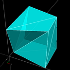
  11  |   0

With more than 2 inputs, the XOR function returns the parity of the inputs. That is, it returns true if the total number of bits in the bitstring is odd. In this tutorial we’ll use 3 bits, chosen mainly to make the decision boundary animation at the top of this article more interesting.

input | output
_______________
  000 |   0
  001 |   1
  010 |   1
  011 |   0 
  100 |   1
  101 |   0
  110 |   0
  111 |   1

This might also be your introduction to the Julia programming language, and represents some of my earliest experiments with the language. Despite the questionable choice of name (necessitating that you qualify it by adding “programming language” almost every time you say it), Julia has some notable advantages.

Developed for scientific computing, the Julia language is ostensibly something of a faster Python, thanks to just-in-time compilation. One interesting feature of the language is that when you see a mathematical definition for a dense layer in a neural network, like so:

𝑓(𝑥)=𝜎(𝜃𝑥+𝑏)

You can write working code that looks very similar, thanks to Julia’s support for unicode characters. It doesn’t necessarily save you any time typing (symbols are entered by typing the Latex command, e.g. \sigma and pressing tab), but it does look pretty cool. The following is perfectly legitimate code in Julia:

σ(x) = 1 ./ (1 .+ exp.(-x))
f(x, θ) = σ(x * θ[:w] .+ θ[:b])
θ = Dict(:w => randn(32,2)/10, :b => randn(1,2)/100)
x = randn(4,32)
f(x, θ)

And returns something along the lines of:

4×2 Array{Float64,2}:
 0.516507  0.482128
 0.568403  0.639701
 0.571232  0.416161
 0.288268  0.546431

If you want to

to OR or X to OR? that is the question.

The exclusive-or (XOR) function is an attractive function to approximate witha simple neural network, both for its simplicity and for its somewhat notorious place in AI research history. In the 1960s a pair of mages of AI nobility proclaimed their revelation that a weighted mapping of inputs to a single output node ( a la Frank Rosenblatt’s Perceptron or the McCulloch-Pitts neuron) could not fit the XOR function, plunging the frontier into chaos and darkness for an epoch. Or so the legend goes. In retrospect it seems that some formal arguments by Minsky and Paypert were taken to be emblematic of all practical implementation. In fact they only proved that dense connections (i.e. non-local weights) and multiple layers were needed to correctly recognize the parity predicate (XOR).

#Separating OR with a straight line is easy, your  eyes will pick out the answer automatically
  
1   x      x
  
  
0   o      x 
    0      1
1  \x      x
    \
     \
0   o \    x
       \
    0      1

# Separating XOR is not so simple, you'll need a curved line to do it. 
1   x   \  o
  ____   \____
      |
0   o  \   x
        |
    0      1

Since then it’s something of a tradition to program an MLP to solve the XOR problem when picking up a new language for ML.

automatic differentiation and software 2.0

We’ll use the automatic differentiation package Zygote from FluxML. If you have used Autograd or JAX before, Zygote will feel familiar, as Zygote is an autodiff package in true “Software 2.0” spirit. You can differentiate over native Julia code including loops, flow control, and recursion. This can have some pretty nifty advantages, for example you can differentiate through a physics model to improve learning for reinforcement learning style control problems. In our case we’ll just differentiate with respect to a few matrix multiplies, and if you’d rather enjoy this tutorial interactively in the form of a Jupyter notebook, visit the Gihub repo.

We’ll use Zygote to automatically give us a gradient to update our NN parameters. This might look a little different if you are used to calling loss.backward() in PyTorch or explicitly programming your own backward pass. Zygote performs the forward and backward pass for us automatically. Unfortunately this meant that I had to call separate forward passes for both training metrics and gradients, but I’ll add an update here when I find a good way to avoid the redundant forward pass call.

lr = 1e1;
x, y = get_xor(64,5);
θ = init_weights(5);
old_weights = append!(reshape(θ[:wxh],  
    size(θ[:wxh])[1]*size(θ[:wxh])[2]),
    reshape(θ[:why], size(θ[:why])[1] * size(θ[:why])[2]))
    
    
dθ = gradient((θ) -> get_loss(x, θ, y), θ);
plt = scatter(old_weights, label = "old_weights");
θ[:wxh], θ[:why] = θ[:wxh] .- lr .* dθ[1][:wxh], θ[:why] .- lr .* dθ[1][:why]
new_weights = append!(reshape(θ[:wxh], 
    size(θ[:wxh])[1]*size(θ[:wxh])[2]),
    reshape(θ[:why], size(θ[:why])[1] * size(θ[:why])[2]))
scatter!(new_weights, label="new weights")
display(plt)

Weights modified according to their gradient.

Now to get started. First we’ll import the packages we’ll use. That’s Zygote and a few others we’ll use for plotting and calculating statistics.

using Zygote
using Stats
using Plots
using StatsPlots

We’ll need both training data and some matrices to act as neural weights, which the functions below will produce for us.

get_xor = function(num_samples=512, dim_x=3)
    x = 1*rand(num_samples,dim_x) .> 0.5
    y = zeros(num_samples,1)
    for ii = 1:size(y)[1]
        y[ii] = reduce(xor, x[ii,:])
    end
    x = x + randn(num_samples,dim_x) / 10
    return x, y
end
init_weights = function(dim_in=2, dim_out=1, dim_hid=4)
    
    wxh = randn(dim_in, dim_hid) / 8
    why = randn(dim_hid, dim_out) / 4
    θ = Dict(:wxh => wxh, :why => why)
    
    return θ
    
end

This next bit defines the model we’ll be training: a tiny MLP with 1 hidden layer and no biases. We also need to set up a few helper functions to provide loss and other training metrics (accuracy). To use Zygote’s automatic differentiation capabilities, we need a function that returns a scalar objective function.

f(x, θ) = σ(σ(x * θ[:wxh]) * θ[:why])
get_accuracy(y, pred, boundary=0.5) = mean(y .== (pred .> boundary))

log_loss = function(y, pred)
   
    return -(1 / size(y)[1]) .* sum(y .* log.(pred) .+ (1.0 .- y)
             .* log.(1.0 .- pred))
end
get_loss = function(x, θ, y, l2=6e-4)
pred = f(x, θ)
    loss = log_loss(y, pred)
    loss = loss + l2 * (sum(abs.(θ[:wxh].^2))    
           + sum(abs(θ[:why].^2)))
    return loss
end

The gradient function from Zygote does as the name suggests. We need to give gradient a function that returns our objective function (log loss in this case), which is why we made an explicit get_loss function earlier. We'll store the results in a dictionary called dθ, and update our model parameters by following gradient descent. The function below defines our training loop.

train = function(x, θ, y, max_steps=1000, lr=1e-2, l2_reg=1e-4)
    
    disp_every = max_steps // 100
    losses = zeros(max_steps)
    acc = zeros(max_steps)
    for step = 1:max_steps
        
        pred = f(x, θ)
        loss = log_loss(y, pred)
        
        losses[step] = loss 
        
        acc[step] = get_accuracy(y, pred)
        dθ = gradient((θ) -> get_loss(x, θ, y, l2_reg), θ)
        θ[:wxh], θ[:why] = θ[:wxh] .- lr 
                .* dθ[1][:wxh], θ[:why] .- lr .* dθ[1][:why]       
        
        if mod(step, disp_every) == 0
            
            val_x, val_y = get_xor(512, size(x)[2]);
            pred = f(val_x, θ) 
            loss = log_loss(val_y, pred)
            accuracy = get_accuracy(val_y, pred)
            println("$step loss = $loss, accuracy = $accuracy")
            #save_frame(θ, step);
       end
    end
    return θ, losses, acc
end

With all our functions defined, it’s time to set everything up and start training. We’ll use violin plots from the StatsPlots package to show how the distributions of weights change over time, using a plot function with the ! in-place modifier to add more plots to the current figure. If we want to display more than 1 figure per notebook cell, and we do, we need to explicitly call display on the figure we want to show.

dim_x = 3
dim_h = 4
dim_y = 1
l2_reg = 1e-4
lr = 1e-2
max_steps = 1400000
θ = init_weights(dim_x, dim_y, dim_h)
x, y = get_xor(1024, dim_x)
println(size(x))
plt = violin([" "], reshape(θ[:wxh],dim_x * dim_h), label="wxh", title="Weights", alpha = 0.5)
violin!([" "], reshape(θ[:why],dim_h*dim_y), label="why", alpha = 0.5)
display(plt)
θ, losses, acc = train(x, θ, y, max_steps, lr, l2_reg)
plt = violin([" "], reshape(θ[:wxh],dim_x * dim_h), label="wxh", title="Weights", alpha = 0.5)
violin!([" "], reshape(θ[:why],dim_h*dim_y), label="why", alpha = 0.5)
display(plt)
steps = 1:size(losses)[1]
plt = plot(steps, losses, title="Training XOR", label="loss")
plot!(steps, acc, label="accuracy")
display(plt)

Weights changing over the course of a training, learning curve shown on the right.

Finally, it’s a good idea to generate a test set to figure how badly our model is overfitted to the training data. If you’re unlucky and get poor performance from your model, try changing some of the hyperparameters like learning rate or L2 regularization. You can also generate a larger training dataset for better performance, or try changing the size of the hidden layer by changing dim_h. Heck, you could even modify the code to add L1 regularization or add layers to the MLP, so knock your socks off and have a go.

test_x, test_y = get_xor(512,3);
pred = f(test_x, θ);
test_accuracy = get_accuracy(test_y, pred);
test_loss = log_loss(test_y, pred);
println("Test loss and accuracy are $test_loss and $test_accuracy")
>>Test loss and accuracy are 0.03354685023541572 and 1.0

testing vs validation

The difference between a test and validation dataset is blurry when we generate data on demand as we do here, but normally you wouldn’t want to go back and modify your training algorithm after running your model on a static test dataset. That sort of behavior runs a high risk of data leakage as you can keep tweaking training until you get good performance, but if stop only when the test score is good you’ll actually have settled on a lucky score. That doesn’t tell you anything about how the model will behave with actual test data that it hasn’t seen before, and this happens often in the real world when researchers collectively iterate on a few standard dataset. Of course there will be incremental improvement every year on MNIST if everyone keeps fitting their research strategy to the test set!

In any case, thanks for stopping by and I hope you enjoyed exploring automatic differentiation in Julia as I did.