How to build an extremely fast analytical database -Part1
In the realm of databases, there are primarily two categories: transactional databases that focus on handling transactions and analytical databases that prioritize analysis. For an analytical database, performance is of utmost importance. In this article, I will share insights on how to create an exceptionally fast analytical database based on CPU technology. (Note: this article does not discuss heterogeneous computing such as GPU or FPGA, nor does it delve into new hardware accelerators like RDMA or NVM.)
This series of articles will explore nine perspectives: precomputation vs. on-the-fly computation, scalability, data streaming, resource utilization, optimization, resilience, architecture vs. details, approximation vs. precision, and performance testing. Through these angles, we will delve into the process of building a lightning-fast analytical database.
Part1: Precomputation vs on-the-fly computation

In essence, databases are primarily involved in two tasks: storing data and retrieving/querying data. When data is written into a database, it ensures data integrity and prevents data loss. When we need to query or analyze data, the database should be able to efficiently and accurately retrieve the desired information. As depicted in the diagram above, when the on-the-fly computational capacity of the database remains constant, there are two major approaches to enhance query performance:
- Precomputation during the database import process: This involves performing certain preprocessing steps to reduce the cost of on-the-fly computation.
- Space-time trade-off during data storage: This approach aims to reduce the cost of on-the-fly computation by optimizing data storage.
These approaches can be further categorized into four main techniques:
1.1 Materialized View
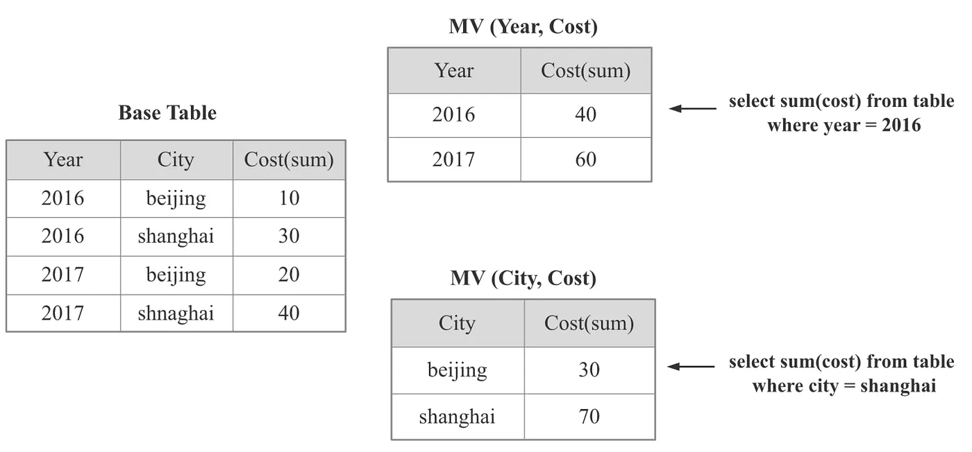
As illustrated in the diagram above, materialized views involve precomputing the results of certain SQL queries and storing them in advance, trading off import latency and storage costs for high-performance querying. Materialized views are a common acceleration technique in OLAP databases. Some examples of materialized views in different database systems include:
- Materialized views in StarRocks.
- Rollup in Google Mesa.
- Cubes in Apache Kylin.
- Star-Tree Index in Apache Pinot.
- Lattice in Apache Calcite.
- Reflections in Dremio.
These techniques aim to optimize query performance by precomputing and storing aggregated or summarized data, reducing the need for on-the-fly computations during query execution.
The key considerations in materialized view technology are as follows:
- Expressing the materialized view model: This involves defining the structure and content of the materialized views in a way that captures the desired data and query patterns.
- Determining which views or SQL queries to materialize: Typically, only a subset of views or queries need to be materialized to accelerate a significant number of queries. The selection process should consider the most frequently executed and time-consuming queries.
- Maintaining materialized views: When the base tables are updated, the materialized views need to be efficiently updated as well. This involves techniques such as incremental updates, support for multiple table materialized views, and handling updates and deletions to ensure data consistency.
- Finding the optimal materialized views for a given query: Determining which materialized views can be utilized to improve query performance requires an analysis of the query’s structure and the available materialized views.
- Query plan optimization with materialized views: Once the potential materialized views are identified, the query optimizer needs to choose the best execution plan by considering the cost and benefit of utilizing each materialized view.
- Balancing query performance, import speed, and storage costs: Finding the right balance between query performance improvements, import speed for maintaining materialized views, and storage costs is crucial. Google Napa, the successor to Google Mesa, has addressed this challenge effectively.
So when is materialized view technology necessary?
- When dealing with extremely large datasets (in the order of billions or trillions) or small-scale clusters (a few nodes or tens of nodes).
- When the query workload involves complex computations, such as joining multiple tables or performing precise deduplication.
- When low query latency is a critical requirement that cannot be achieved solely through on-the-fly CPU-based computations.
- When there is a need to optimize query performance in the face of significant computational challenges.
- When the benefits of materialized views outweigh the associated costs, such as storage and maintenance overhead.
Both Google Mesa and its successor, Google Napa, heavily rely on materialized views due to the scalability and performance benefits they provide in handling massive datasets and complex query workloads. However, if the dataset is not large, cluster resources are abundant, or the queries are not particularly complex, relying on on-the-fly computations may be sufficient and materialized views may not be necessary.
1.2 Aggregation Table
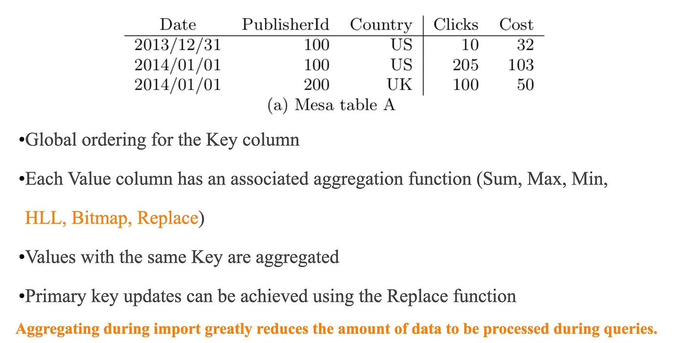
In OLAP systems, there is a distinction between dimension columns and metric columns. Pre-aggregation, in this context, refers to the process of aggregating data from multiple rows into a single row during the data import phase. The values in dimension columns remain unchanged, while the metric columns are aggregated based on the associated aggregation functions. By performing pre-aggregation, the original dataset, which could have been billions of rows, can be reduced to just a few million rows. Processing a few million rows is significantly faster than processing each individual row separately.
Pre-aggregation is a common technique used in OLAP databases for performance optimization. Some examples include:
- Aggregation models in StarRocks.
- Aggregation models in Apache Druid.
1.3 Index
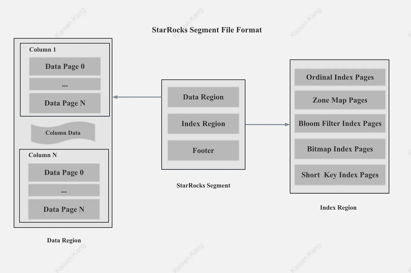
An index, in the context mentioned, refers to metadata or data structures outside the original dataset that are used to accelerate the retrieval of specific values or offsets within the dataset. Indexing is generally categorized into lightweight indexes and heavyweight indexes. Lightweight indexes include ZoneMap indexes (Max, Min, Has null), prefix indexes, while heavyweight indexes include SkipList indexes, B-Tree family indexes, Hash indexes, Bitmap indexes, Bloom Filter indexes, among others. This blog will not delve into the specific technical details of indexing. However, the challenges of indexing can be summarized as follows:
- How to automatically select and build different types of indexes based on data scale, data types, and data cardinality.
- When multiple indexes can be used for a single query, how to adaptively choose the best index.
- Balancing between write speed, storage costs, and query performance.
In summary, the purpose of indexing is to avoid reading a large amount of irrelevant data from the storage layer, thereby speeding up queries. It is an essential means of acceleration in database storage layers.
1.4 Cache
Cache is ubiquitous in computing, and if we know that a particular query will be queried multiple times, we can cache the first occurrence of that query. Caches can exist at various levels, such as the operating system’s Page Cache, the database storage layer’s cache for files or pages at the block level, and the database computing layer’s cache for partitions, segments, and result sets. The challenges of caching include avoiding frequent cache evictions and ensuring cache hit rates. There are numerous articles discussing caching in detail, but this blog will not delve into it extensively.
1.5 Generated Column

As shown in the diagram, when there is a need to accelerate certain computationally intensive expressions or speed up queries on specific columns within complex types (such as Map, Json, Struct), one approach is to materialize the computed results of those expressions or store specific columns of the complex types. This allows for automatic query rewriting during retrieval, achieving transparent query acceleration.
In the next article, we will discuss how to build an ultra-fast database from the perspective of scalability.
