Blooming China Pink in the Midst of Precalculus
Introduction
Roses are red, and violets are blue, but have you ever realized that mathematical equations can also create intricate, beautiful patterns that captivate our eyes just like flowers do? In mathematics, there are mainly two means of representing the mathematical relationships of two variables in a graph. The Cartesian plane, also known as a rectangular coordinate system, may be more familiar to us. It consists of two axes of x and y that are perpendicular to each other. While using cartesian graphs can be beneficial in identifying the relationship between the two variables, it cannot effectively manifest the intricate shapes of flowers. Therefore, the method that we investigate in this project is a polar coordinate system and polar graphs. The polar coordinates are represented by the pairs of the angle from the reference direction and the distances from the pole. Polar graphs are able to depict circular patterns since it uses angle as one of the variables. Also, by applying many concepts and rules from trigonometry, we are able to illustrate an intricate shape that closely resembles the circular patterns in nature.
The polar graph project has been a revolutionary mathematical project gradually being solidified as a tradition of Dr. Tong’s Honors Precalculus class. From 2018–2019 period, Dr. Tong has been raising the bar every year as students actively investigate new innovative methods of illustrating nature through polar graphs. Its theme started from flowers to architecture, to vegetables, and back to flowers this year. However, there was one additional requirement that raised the difficulty of the project to a different level: animation. This year, we had to create a dynamic animation of our flowers blooming. This meant that either we had to create a few hundred frames or find an alternative mean to portray the movements of flowers. This project had led to moments of devastation, moments of inspiration, and moments of pride and joy. Here is my process.
China Pink

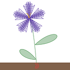
The flower that I chose was China Pink. Dianthus Chinensis, also known as China Pink, is a flower native to China that grows from 6 inches to 30 inches. It is a short-lived perennial popular for its colorful, flat flowers with fringed petals and a dark central eye. China Pink blooms over a long period from late spring to summer, and the flower’s colors can vary from white to red, often in a combination of those two colors. While its delicate color patterns perfectly persuaded me to choose it, my frequent acquaintances with China Pink back in my hometown led me to the final decision of choosing it.
Preliminary Aspects: Frames vs Sliders vs Groups
Prior to designing the animation for China Pink flower, I had to decide which method was the most effective to illustrate various graphs in a dynamic animation since this would alter how I would design my polar graphs.
Frames

The first method that came to my mind was to create numerous frames and utilize stop-motion videos to create an animation. However, after experimenting with a simple polar graph and attempting to create dynamically animated frames, I realized that there will be numerous difficulties in adjusting the polar graphs for each frame. Also, I estimated that hundreds of frames would be needed to depict the scenes I was planning. And so, I searched for a different approach.
Sliders

Another way that I investigated was using the slider function in Desmos. Like in coding, Desmos allows the users to define a variable and create a slider to gradually increase or decrease the variable’s value. Also, I found out that Desmos provides 4 different modes in how sliders can change the value of a variable. There are “loop forward and back,” “repeat in one direction,” “play one time,” and ” and “play indefinitely” modes. There is also a speed mode that I could adjust the speed of how values changed. And so, I attempted to directly animate the polar graph by multiplying a variable to the equation to control the size or the number of petals of the flower. However, a shortcoming of using sliders was that I wasn’t able to fully control the motions of the blooming. Because the sliders continuously changed the values at a constant speed, the blooming of the flower was not coordinated and didn’t resemble a realistic blooming of China Pink.
Organs
Another way that I found was having separate animations for each of the organs in the flower. For instance, I would animate only the flower petals blooming and separately animate a stem growing. This way, I would be able to combine separate animations into one animation that resembles the blooming of China Pink.
Final Decision
After considering the pros and cons of three different methods, I decided to incorporate every method into the project. After designing the polar graph for the final flower, I realized that some portions of the graph could be depicted using sliders and that other portions of the graph such as linear graphs had to be depicted using stop-motion frames. Also, I organized the project into different groups representing each organ of the flower or a scene. This way, the growth of the flower was coordinated perfectly.
Progress
Step 1: Final Flower

The first thing I had to do was to draw the final flower. Although it would appear in the last order of the animation, it was the most important component. And so, it was best to design the final flower and work on other organs according to the reference of the final flower. First, I needed to make the main body of five petals. From a basic form of r=a*sinb𝜽, the b value determined the number of petals in a rose curve. And so, I put the b value as 5 but then realized that if I increased the number to 5.1 and adjusted the domain, I could produce a slightly rotated flower addition to the original graph. Therefore, I made 3 graphs of b value as 5.1 and adjusted their rotation by controlling the values added to theta. By doing that I was able to depict a 5 petal flower with curvy edges at the end. Additionally, I found out that the outer edges of each petal were sharp lines, features that may be difficult to depict from a typical polar equation. Therefore, for those portions, I had to use linear equations to depict the sharp edges. A typical linear graph in Cartesian coordinates would be y=ax+b or ax+by-c=0. However, I needed to represent it in the form of a polar graph. And so, it was necessary to convert the linear equations in rectangular form into polar coordinates. To do that, I derived from the two conversion equations: “x=r*cos𝜽 and y=r*sin𝜽.” When I replaced x and y in a standard linear equation, it was depicted as r*sin𝜽 = a*r*cos𝜽+b. When this equation was written for r, the equation of r= b/(sin𝜽-acos𝜽) was derived, with a representing the slope of the line and b representing the y-intercept. With this equation, I was able to depict the outer edges of the flower by adjusting the linear graphs’ slopes, y-intercepts, and domains.
Step 2: Blooming

After completing the final flower, the first scene that I worked on was the blooming scene. In this process, I had to come up with how to transition from a simple circle depicting a bud into the final flower. I divided the scene into two parts: the first part by using sliders and the second part by using numerous frames. The first part illustrated the simple circle depicting a bud to the final flower that did not have the sharp edges represented by linear graphs. The second part only included the sharp edges of the final flower growing gradually. The reason why I had to use sliders for the second part was that it was difficult to dynamically move the linear graphs altogether. Unlike a typical polar graph that can change its size or number of rotations using a variable, a linear graph in polar form cannot be animated with a single variable. And so, I created 4 frames for the second part, which show a gradual increase in the sharp edges. Then, I worked on the first part from a simple circle into the final flower with an absence of sharp edges. First, I drew a simple circle depicting a bud using the equation r<z and set z as a variable changing accordingly to the slider. From this, I was able to represent a small bud growing from the center. Then, I replicated the final flower’s equations and adjusted the rotation of the polar graph by adding certain values to the theta. After this, I multiplied a variable of a slider to animate the growing scene. This was to represent 5 small petals emerging from the small circular bud. Then, I multiplied additional variables to the final flower’s equations to depict the final petals growing. One more thing was needed for completing the first part of the blooming scene. I needed to show the pistils and stamens growing from the flower. Since pistils and stamens were slightly curved lines, I decided to depict them using a polar form of a parabola. Converting the rectangular parabola equation to polar form was not a difficult procedure as the equation was converted to r=a/(b+sin𝜽) form after substituting rcos𝜽 and rsin𝜽 for each x and y value in the original equation. Then I multiplied r=a/(b+sin𝜽) to cos(t) sin(t) separately in the parametric equation to represent each of the x and y values. Finally, after adjusting the horizontal and vertical translation of the parametric equation, I inputted a variable of a slider in the domain of the parameter t to depict the pistils growing.
Step 3: Stem Growth & Leaves

The next scene that I needed to depict was the scene illustrating the growing stems and leaves. First, to depict the stem growing, I used a parabola equation that was convex to the upside. Just like the pistils and stamens from the previous scene, the parabola rectangular equation was converted to r=a/(b+sin𝜽) form. Subsequently, I adjusted the domain of theta using the variable of a slider to illustrate the stem growing. Next, I had to create two leaves that would grow from the central stem. For the shape of leaves, I used the equation r=sin4𝜽 and convert the equation to parametric form to translate them to the right position. Then, I decided to use the same slider variable that coordinated the stem growth since it would be much more efficient than having separate sliders for each component. Therefore, I multiplied the same slider variable to the domain of the parameter of the leaves to represent the leaves growing.
Step 4: Seed Drop

Although most of the polar flower animation showed flower blooming and stem growth scenes, I decided to expand further and add a seed drop scene to add more dynamic elements to the animation. The notion behind the seed drop was easy compared to the intriguing effect of the scene as an effective introduction. To illustrate a seed, I investigated the limacon shapes of polar graphs, which added a coefficient to the changing value of cos𝜽 or sin𝜽. After adjusting the coefficients to depict the limacon shape that I wanted, I converted the polar equations into a parametric coordinate by multiplying r, which was a+bcos𝜽 to either cos t or sin t for each x and y value. By converting the polar equation to a parametric coordinate system, I now had the ability to translate the equation both vertically and horizontally. And so, by creating a variable using a slider and adding it to the y value of the graph, I was able to depict the seed falling.
Step 5: Raindrops

After completing the seed drop scene, I started to think “If dropping a seed is possible, why would dropping water droplets not be possible?” And so, I decided to add a rainy scene to my final animation. In creating the shape of a water droplet, I used the same structure of the limacon equation as the seed. However, I had to adjust the ratio of the coefficients to finally create the shape that I wanted. After the conformational shape of the rain droplet was set, I replicated the equation 8 times to have numerous rain droplets falling. Then, I adjusted their horizontal translation to make each of the droplets to be in different horizontal positions. Now, it was the most important part in depicting the scene: vertical translation. To create the dynamic fall of water droplets, I added separate variables to each replicated equation. This was when the “repeat in one direction” became useful as I was able to make the water droplets constantly drop in one direction.
Animation

After completing all the graphs necessary for every scene in the animation, it was time to assemble all these equations into one beautiful animation. Initially, I considered recording the animation in one take, which means not using any video editing to assemble the scenes. However, for fluidity and transition between the scenes, I decided to record each scene separately and assemble them using a video editor. Since most of the scenes used sliders to depict movements, it was easy to record by just clicking the slider button. However, for one scene in the blooming scene that requires numerous frames, I had to screenshot each frame and combine them to create a small stop-motion animation. Lastly, I added sound effects for each of the scenes to also capture auditory sensory as well as visual sensory.
Reflection

Before I started the project, I had many doubts about myself. I was unable to estimate how much effort and time would be required to not only create a beautiful polar flower but also create an animation that may require up to hundreds of frames. And so, I was not confident to start the project initially. However, after investigating deeper into the principles behind the polar graph and making the first frame of my animation, I began to gain more confidence and enjoyment while carrying on with the project. On the way, I was able to discover many mathematical concepts that I failed to grasp months ago when I was learning polar equations. Also, I discovered more efficient ways of graphing or animating that I couldn’t come up with at the start of the project. And so, I was able to finish my project on time and further expanded my project by adding additional scenes to the animation. Through this project, I was not only able to reorganize my understanding of polar equations but also were able to develop a new aspect of viewing the natural world through the eyes of mathematics.