Generative AI: Malfunctions, Imperfections, Irrationality and Expression

A week or two ago I was speaking with a fellow machine learning engineer. They were telling me that they didn’t believe that AI could truly ‘create’. That there was an essential human element that was lacking from a model’s output. That there was no intention. No decision. Only algorithm. And that an unsupervised algorithm was only a sophisticated set of instructions that could retain and display learned information but that the output was not an expression. At most a disguised regurgitation. They explained the output as only a product, a result. They got me thinking about what the output was a result of: Should the result be considered a product of the model’s functionality? Maybe the mathematical construction of the model? Or perhaps it was a product of the coding language used and its native compiling methods? Or is it a product of the deep learning engineer who learned the coding language, studied the model’s functionality and construction, and intentionally tuned the hyper-parameters to its most optimal state for the model to train?
We both couldn’t deny that when using deep learning models, the experience still feels novel. There’s an excitement when the model finishes the training phase and outputs text, midi patterns, images or predictions. In my experience, it always appears new. Sometimes comical, non-sensical, or incoherent; sometimes outright wrong, but other times the output is poetically sophisticated, harmonically functional and uniquely composed with a clear influence of the works it was trained on. As if the model had really grasped underlying patterns in the decision making process, the expressive signature, of the creator it was trained on and made the next logical iteration of that creator’s process.
Our conversation made me consider what expression was. Can human expression be isolated and represented in data? If so, can’t a model retain the principles of that data’s structure? They rebutted with the example of market analysis to suggest that what is retained by a model is not the expression itself, but rather an insight describing the expression. An insight categorizing and understanding the expression. But not an insight making the expression. Let’s say we gather a data set on a marketing campaign. The data may well inform us where to invest our marketing budget, between which platforms to maximize our ROI based on current cultural practice — but can the model truly understand the consumer or cultural context of why the market campaign is working or not? Can it isolate and retain the ethos of the market? Can the model make the decision or anticipate unexpected social trends? They asked me to consider why a model can’t predict if or when a tweet, or some youtube video will go viral. They asked me to consider what is missing.
After reflecting through a few minutes of silence, I admitted I couldn’t articulate but innately understood what they were getting at. They simply said: “Irrationality” Maybe the model can predict the next logical iteration of a process, but humans do not follow a logical path with absolute precision. People change, and sometimes unexpectedly. As the loss function cascades down to zero and accuracy achieves a position close to one hundred precent, the model becomes more and more enclosed in a narrowing path of rationality and remains a process embedded in the logical context of its training.
Interestingly enough I found myself in another conversation with a fellow composer and producer not too long after. Convinced with a satirical pessimistic tone, they hyperbolized that there would be no human composers in the future. No human authors. No human philosophers. No human scientist or doctors. No human police or soldiers. That the state of our emerging modern societies would be automated to a point of social classes defined by owners of the AI, operators of the AI and those subdued and entertained by the AI. While the sarcasm was noted, they’re not the first to hold this idea. Entire cyberpunk genre’s were developed from this notion. Whether it be 1999’s The Matrix or 1921’s R.U.R the concept of ‘The Second Renaissance’ has been part of our social lexicon for sometime. Reminiscent of aliens, monsters born of advancements in science and superstitions or the destruction of nature from the industrial revolution — the concept of technologies and unknowns dominating with anthropomorphic motives, in my opinion, can largely be traced to not understanding. Then reacting with a defense mechanism.
Both of my friends might laugh at one another’s position believing the other, respectively, is too optimistic and underestimating or too pessimistic and overreacting. In some sense, it’s a trade off. Rather than take a side, I wanted to venture into the curiosity with an aim to find the middle ground. A place where AI is an extension of human intelligence. A tool to enhance how we interact with ourselves and our environment; not a tool of dependence or oppression.
In 1956, at University of Illinois at Urbana-Champaign, Lejaren Hiller and Leonard Isaacson developed the first work composed by AI. It was titled, ‘Illiac Suite for String Quartet’. The work is made up of four movements, each a product of an experiment. Illiac is an acronym for: Illinois Automatic Computer.
The first experiment focused on setting an algorithm that resulted in a Cantus Firmus. Cantus Firmus, meaning ‘fixed song’ refers to a process where a composer uses a pre-existing melody as the outlining structure of the work, as well as the structure for the interior voices in order to achieve polyphony. It is a technique that is replicable and often used to teach species counterpoint.
Movement 1 below:
The second experiment is an algorithm focused on resulting four voices, where each voice follows a set of rules.
Movement 2 below:
The third experiment is an algorithm that results in varied rhythm, dynamics and playing instructions.
Movement 3 below:
Finally, the fourth experiment is an algorithm that I like to call a musical expression of probabilistic models.
Movement 4 below:
The interesting thing about this Suite, is not that Illaic created new music. Here I would have to agree with my first friend. What is occurring is that the Illiac is precisely executing an algorithm set by Hiller and Isaacson. Rather than the computer creating, it is more so translating a defined set of rules into musical expression. Each experiment is focused around techniques and aesthetics that were very prevalent in academic music during modernism. In a sense, a human would have probably written something similar, but perhaps the Illiac just wrote it quicker through a series of automated process. Here, the computer isn’t creating, only executing.
Not until David Cope in the1980s do we get Emmy. Emmy is a nickname for Experiments in Musical Intelligence. For Cope, Emmy is about style simulation. Recreation of what already exist. Distilling a style into an algorithmic replication. There is an excellent interview with him called: Composing with Algorithms: An Interview with David Cope. He essentially talks about music in terms that it is already a natural system. We organize it into styles. Styles become records of operations within music that emerged in varying cultural contexts. The emergent operations popularized at any given time are more so an expression of cultural aesthetic.
When asked by Keith Muscutt, “How would you define algorithmic music?”
Cope replies, “An algorithm is a step-by-step recipe for achieving a specific goal. Breathing, heartbeats, blinking, and so on, are all naturally occuring algorithms that help keep us alive. DNA, the building block of life, represents another good example of a common algorithm”
When asked, “In your opinion, who are the most important historical algorithmic composers?”
He goes much further than 1950’s Illiac.
Cope replies, “When I consider the history of algorithmic music, I think almost immediately of Guillaume de Machaut, the 14th-century composer who plotted isorhythms — different lengths of interlinked pitches and durations — …..I also think of J.S. Bach, whose fugues, canons and similar algorithmic music form a substantial part of his musical output”
At another point Cope speaks of how Xenakis used mathematical principles to develop his patterned stochastic music. Often using grids rather than traditional ledger lines. Further more, there is something I find to be one of the most insightful interpretations of music in this interview. Cope says,
“Algorithms can be as vague or explicit as those who invoke them desire. Classical sonata-allego form is an example of a vague algorithm, where the general types of materials are denoted, but not the actual musical materials themselves. On the other hand, Baroque figured bass is a fairly explicit algorithm….should be followed precisely”
Cope interprets the creative process as an algorithm itself. Music in his interpretation is a medium to express our creative algorithms. The music we make becomes an output of our human interaction with the natural system of music. Resulting compositions reflect structural decisions within our creative algorithms. In this sense, a deep learning model could distill the structural principles a composer leaves in their work. The composition is a sequence in time. The musical patterns are the data. Converting it to an input to train a model doesn’t seem that far out.
Before I talk about how 5 LSTMs and a Linear SVC get involved, I want to suggest an idea. Returning to the initial question. It seems evident that generative AI is a combined expression depicting how the model works, how the architecture is structured, how the data is used to train it; and the engineer who tunes the hyper-parameters. For generative AI to be a collaborative extension to the “algorithm” of human creativity seems to be the middle ground. The question becomes, which aspects of the creative algorithm do we want to experiment automating when collaborating with AI?
When talking about machine learning models, there is a concept that is irresponsible to neglect when considering the evaluation of a model’s performance. The concept of bias / variance trade off. For those who need a refresher, I’ll briefly explain.
Bias
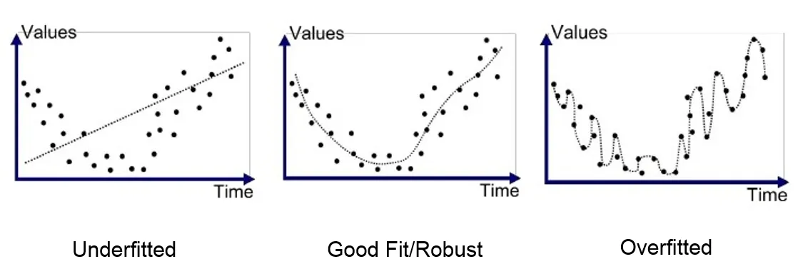
Bias is the difference between the average prediction of the model and the correct value. Having a high bias is also known as underfitting. This means that the model is over generalizing the training data and is unable to detect the underlying pattern within the dataset. Therefore, is inaccurate when predicting on test data.
Variance
Variance is the variability of the model’s prediction for a given data point. Having high variance is also know as overfitting. This means that the model performs very well with the training data. Actually, too well. So much so that it also inaccurate when predicting on the test data, but in the opposite fashion. Rather than not detecting an underlying pattern in the training data, it is so tightly fit to the training data that it cannot predict what is not already show to it.
Bias / Variance Tradeoff
The trade off is an achieved balance between simplicity and complexity of parameters. If the model is too simple, it will be underfit and over generalized. If the model is too complex, it will be overfit and too specific. Finding a balance between the two will produce a model that is more accurate. Detecting the underlying pattern in the data but also generalized enough to predict something that it has not already learned.
How does this apply to Generative AI? Let’s stack another concept on this. High Bias as more generative and High Variance as more replicative. In this sense, a generative AI would be a model that outputs something similar the composer it is trained on, but if passed through a classifier, not able to be classified as the composer it is trained on. Like a musician who absorbs influence, yet manages to generate their own algorithm. Replicative, in this sense, would be an AI similar to a model that if given the beginning of a piece of music, would output a replica of the composer’s piece as it is already written. Somewhat like a performer who is lost on their instrument without sheet music in front of them. Unable to produce anything without explicit instruction.
The trade off, here, is the balance achieved when the model can produce a new composition in the style of. Or as David Cope might think, a new composition in the operation of the composer it was trained on. Meaning, when passed through a classifier, the piece would be classified as the composer the model was trained on but, would result in a composition that the composer never wrote.

Thinking of the initial conversation with the fellow machine learning engineer, I would say: intentional malfunctions, celebrated imperfections and accepted irrationality — built in margins of error as methods to achieve AI expression.
Collecting Files
I chose to go with MIDI files for a few reasons. In a technical sense, MIDI would be easy to convert into model inputs. But in a theoretical sense, having the model learn MIDI is analogous to having a composer learn sheet music. In this experiment, I did not want to simulate a performance, but rather simulate the act of composing.
To obtain the files I used four libraries:
import requests
import re
from bs4 import BeautifulSoup
import wget
I scrapped from three websites. The first was Piano Midi Page. The second was Midi World. The third was Classical Archives. From each site I collected as many MIDI files as I could for five composers: Bach, Beethoven, Chopin, Debussy and Ravel. For example, to pull all the Chopin MIDI files from Piano Midi Page, I built this simple function:
This function will pull each piano MIDI file for each composer that you set. Try it out.
Exploring the data in a Composer’s Style
Once I had a dataset for each composer, I used libraries PrettyMIDI and Music21 to visualize and explore the bodies of work. Here’s an example of the visualization. Similar to a piano roll read out that you might find in a DAW, below is a MIDI representation of Chopin’s Op. 9 №2 in Eb. We can use this to obtain a snapshot of the overall structure and form of the piece.

But what could we learn from the composer’s body of work? How would the results from one body of work compare to another, and where would they contrast?
Chopin’s Harmonic Tools
Below is a set of visualizations of what Key, Pitch, PitchSet and Interval Vector and the use count.

For those not familiar, the reason Pitch axis is 0–11 is because the chart is abstracting pitch out of register into PitchSet where 0 = C and 11 = B, with all twelve pitches in between. Some argue that abstracting away octave diminishes the analysis. The argument has merit, but, in this exploratory stage, the insights we are after can still be derived without acknowledging register. The first thing I see here is that Chopin used these three pitches the most: Eb, Ab, Db. Being familiar with Chopin’s work, I’m not surprised with that. Many of his pieces are written in a flat key. However, I do find it interesting that the three pitches most present in his body of work could be stacked to make an undefined mode of a Db9 chord or interpreted as one of the most common progressions in all of music: ii-V-I

Initial glances here tell me the keys used in his body of work are evenly spread in between key names with accidentals and natural key names. There are twenty-four different keys he is activating in his works. Ab being the most common. With that information, it might be more appropriate to look at the pitch count as representing not, ii-V-I, but rather iv-V-I. Also, maybe it would be best to interpret the three pitches as an undefined mode of an Ab11chord. Additionally we see that out of the twelve Keys he uses and equal amount of major and minor modes, but engages with more minor modalities than major.
Lets move on to Pitch Set and Interval Vectors


Both of these graphs are hard to read and essentially tell us one main bit of information. Chopin used a lot of different types of chords. This tells us that his music was very colorful and made use of many different, unique harmonic quality combinations. The immediate suggestion I interpret is that one of the defining characteristics of Chopin’s music is going to be is harmonic and melodic structures. With out getting too lost in music theory, lets contextualize Chopin’s music, historically. He is an iconic Romantic composer. Following Beethoven, whose work may be considered the transition between Classical into Romanticism, Chopin is one of the earliest composers to explore melodic chromaticism and mixed modal progressions that pass through elegant dissonance and dismantle the pillars of functional harmony. All while retaining a poetic balance. His tools are not as far out as the second school of viennese, but his operations are distant from the mechanics of Bach’s harmonic tools. And when we look at Bach’s Harmonic data, it displays that difference.


Immediately it is clear that Bach gravitates to key centers, is using less chord types, remaining in smaller intervallic structures and writing more consistently in natural key names; primarily in D Major, D minor, G Major and C Major. However, there is something interesting about about these three key names, mode excluded. D, G, C has a connection to Eb, Ab, Db. At the core of each composer’s body of work is the same intervallic structure. That is to say: both <Eb, Ab, Db> and <D, G, C> are instances of <ii-V-I>.
Now this is only two composers, and to go further into this, I’ll have to wait to write another blog focused more on musicology and the history of western music to test out this hypothesis. However, I find this pattern interesting. Perhaps Cope would say that <ii-V-I> or <iv-V-I> and both an 11th chord and 9th chord have a lot to do with the DNA of western music.
One last thing about historical context. Read Ross W. Duffin’s How Equal Temperament Ruined Harmony (and why you should care). The basic insight of that text: instruments now and instruments then did not access the natural system of music in the same method. Based on different tuning technologies that instrument engineers used, it was a different sonic experience both limiting and opening different musical activations.
Models and Evaluations
Earlier I mentioned 5 LSTMs and a Linear SVC. Below is the visual representation of the my final model and evaluation flow.

In short, I used each composer’s body of work to train a single LSTM. Then used the entire body of each composer’s work to train an SVC. I wanted to build both an AI model that could compose, then a classifier that could evaluate the work of each model. Having a separate classifier that evaluates the composition allows me to experiment with the hyper-parameters of the LSTM in search of the generative/replicative trade off that I wanted to collaborate with. Just because I have a high loss function during a training session might not necessarily mean an outside classifier can’t recognize the output as the composer that trained the model.
Why Input Matters
My first attempt at this was comical. Listen to result.
The only thing this model learned after roughly eight hours was to predict Ab. So in a sense, it learned the most used key in Chopin’s body of work, but did not learn anything about how Chopin sequenced his pitches. There seemed to be an attempt in the beginning with the flourish of seemingly random notes. But when we take a closer look, the pitches are: F, Gb and A. Certainly not excusing this poor example, but these pitches do make some sense and other than A all fall within the key of Ab.
How did I get here? Two problems in my process. First, how I generated the input for the LSTM and secondly, how I built the LSTM.
Let’s see why my input didn’t capture accurate sequential data.
After parsing the pitches, transforming them in to integers, isolating the patterns and normalizing the input — I’m left with a vector of sequences and pitch relations. Other than over generalize the learning process, there is another thing to observe about the model’s output. Listen to how mechanical the rhythm is. Each note is exactly the same duration and each offset is mostly one after the other. There are vey few instances of where notes occur at the same time. Let’s imagine that this model did learn a more diverse process of predicting notes. There would still be a pretty big problem if they hardly every occurred simultaneously. That type of model would only be able to output melody but completely miss harmony.
The deep learning model’s architecture was a total of 3 LSTM layers and, 3 drop out layers, 2 Dense layers with an activation layer using softmax and compiled with categorical cross entropy as the loss and an rms prop optimizer.
Here’s the summary.

It turns out for the model to understand polyphony and rhythmic data, duration and offset are crucial.
Below is an image depicting how I converted the midi data into a matrix that accounted for duration and offset. In this example it is referring to Ravel’s midi data. The process worked the same for each composer though.

The matrix is 128 x 300. The y axis accounts for all the notes possible 0–127. The x axis is time. Where there is a 1, the note is on. Where there is a 0, the note is off. When a 1 is followed by .5, the note remains on for the entirety of its duration. Once the note ends, a 0 is put in place to represent that the note is again off. This is analogous to interpreting the matrix as a piano roll. In order to normalize the input, there are 300 steps per matrix. If a piece is divided into such that its final matrix does not equal 300 steps, then the rest of the matrix is padded with rests in order to fit the shape. This allows for the model to not only learn the note’s position and its duration, but also to understand their position in relation to each other as chordal intervals and progressive intervals.
I changed the deep learning architecture by adding more layers of activation and dropout, introducing layers of batch normalization, and flattening, changing the optimizer to stochastic gradient descent, specifying the learning rate as well as adding in a handful of layers of leaky relu and tanh functions in order to better control the LSTM signals and memory gates between layers. In addition, in order to amplify attention to significant steps in a composer’s musical patterns, I set the model to use 15 steps in the matrix to predict the next. Further more, I took advantage of keras’ RepeatVector layers and Permute layers to build out and control the feedback loop within the model. This was to optimize the model’s select and ignore gates.
The model summary below:
AI compositions are at the bottom of the article.
As for the Linear Support Vector Classifier, I did not use matrices at all. Rather I converted the midi into xml files and treated the musical literature as text literature and implemented NLP. I did this by taking the chord sequences in a composer’s work and transforming them in ngrams. In a high dimensional sense, this image below describes the process.

To do this, there are essentially two steps after converting the midi into numerical representations:
- Use the twelve tone PitchClass, in the form of a list, to build a function that can detect the distance and abstract the intervallic relation in PitchSets
- Make an index of 192 chords and label each chord from 0–191. Then use the chord index to identify the chords and represent the sequences in a lists of numbers.
Let’s dive into some intervallic mathematics to show how this can be done.
#  12 tone scale in pictchclass
roots = list(range(12))
print(roots)
output: [0, 1, 2, 3, 4, 5, 6, 7, 8, 9, 10, 11]
Okay, cool. We have the twelve tone scale. Now let’s look at a problem and see what we can do to solve it.
Given two notes, what is their intervallic relation?
We are going to start with A and Eb, and Ab and D.
Here are the two sets of notes given as numbers: (9, 3) & (8, 2). First it’s important to note that both PitchSets contain equivalent intervallic distances between PitchClasses. So lets focus on (9, 3) and come back to (8, 2)
We are asking, what is the relationship between PitchClass 9 and 3? A diminished fifth is the answer. A diminished fifth has an interval of six steps. In other words, a diminished fifth is equivalent to PitchSet <06>.
Here’s the solution:
(roots[9-6:]+roots[:(9+6)%12])[6+3], (roots[9-6:]+roots[:(9+6)%12])[6-3]output: (0, 6)
The variable roots = [0, 1, 2, 3, 4, 5, 6, 7, 8, 9, 10, 11]
Below is a notebook that takes you step by step to arriving at this line of code.
Above, this allows us to take converted midi data and see what interval qualities are at the heart of the work. Similar to what is happening under the hood with Music21, this allows us to extract this information and train the Support Vector Classifier.
Secondly, to make the chord index, I took the twelve tone system and multiplied the abstracted system by the sixteen most common chord qualities. Essentially 12x16 = 192 PitchSets. I did not convert the PitchSets to their PrimeForm, rather left them in NormalOrder in order to retain information about what key the composer was using in addition to the intervallic qualities.
Below is a notebook that takes you step by step to building the index.
Now let’s look at the Support Vector Classifier itself. When using the chord ngrams and these parameters for the SVC:
Parameters: Loss: ‘Hinge’ Penalty: ‘L2’
the model reached a performance level of:
Fscores:Micro-Weighted: 97.41%Macro-Weighted: 95.4%

Note: I had to let go of Ravel during the classification training due to how little works I was able to retrieve of his. I was still able to to make an AI_Composer model, but the music was not enough be effective in the classifier.
While I was happy with the result of the classifier’s training, my fellow machine learning engineer friend tasked me with the question: “If incorporating rhythm had a positive affect on performance of you’re AI_Composer, shouldn’t it increase accuracy here?”
It was a good insight. After making ngrams on the durations and offsets of each chord and training the classifier on both chord ngrams and duration ngrams, I was able to push the accuracy to nearly 100%. With same parameters, the model’s performance jumped to:
Fscores:Micro-Weighted: 98.63%Macro-Weighted: 98.15%

Lastly, in order to not leave Ravel out of the mix completely, I made a binary classification model that was trained to classify whether a composition was from a Ravel or Debussy AI_Composer. Using the same parameters and method of generating inputs, I reached a model that performed:
Fscores:Micro-Weighted: 91.67%Macro-Weighted: 90.0%

Choosing SVC seemed like the obvious chose do to the nature of how the model interacts with features per data point, but I also evaluated the performances of Logistic Regression, KNN, Multinomial Naive Bayes and a Multi Layer Perceptron Classifier. All of them did well, but The Support Vector Machine was consistently the most accurate through out the different variations of ngram types and different hyper-parameter settings.
Each AI_Composer model is set to generate a new piece each time the code is run. This is due to using a random generator for the inputs to set the generative process in motion. Below are 5 that I felt were interesting…
Chopin_Bot:
Ravel_Bot:
Bach_Bot:
Beethoven_Bot:
Debussy_Bot:
When passed through the classifier, the AI’s output is classified correctly between, roughly, 57% — 70% of the time. The margin of error built into the AI model could be seen as a deviation, or could be interpreted as the AI’s own creative decision making. The expression of the AI. Or perhaps an expression of the engineer. However you decide to think about it, the SVC could detect to some degree, an AI’s output had something in common, with the composer’s data that trained it. But these 5 examples are times when the SVC misclassified the compositions.
There is something mechanical when listening. I can tell that it is not a human playing. But I wonder what it might sound like to sample these works and use them as a starting point for a project? Or to print the sheet music and have a human perform them rather than a computer? How might the model and I be able to work together?