Object Detection with Transformers
A complete guide to Facebook’s Detection Transformer (DETR) for Object Detection.
Introduction
The DEtection TRansformer (DETR) is an object detection model developed by the Facebook Research team which cleverly utilizes the Transformer architecture. In this post, I’ll go through the inner-workings of DETR’s architecture to help provide some intuition on it’s moving parts. The colab notebook accompanying this tutorial can be found here:
Below, I’ll explain some of the architecture, but if you just want to see how to use the model, feel free to skip to the coding section.
The Architecture
The DETR model consists of a pretrained CNN backbone (like ResNet), which produces a set of lower dimensional set of features. These features are then formatted into a single set of features of and added to a positional encoding, which is fed into a Transformer consisting of an Encoder and a Decoder in a manner quite similar to the Encoder-Decoder transformer described in the original Transformer paper (http://arxiv.org/abs/1706.03762). The output of the decoder is then fed into a fixed number of Prediction Heads which consist of a predefined number of feed forward networks. Each output of one of these prediction heads consists of a class prediction, as well as a predicted bounding box. The loss is calculated by computing the bipartite matching loss.

The model makes a predefined number of predictions, and each of the predictions are computed in parallel.
The CNN Backbone
Assume that our input image xᵢₘ of height H₀, width W₀, and three input channels. CNN backbone consists of a (pretrained) CNN (usually ResNet), which we use to generate C lower dimensional features having width W and height H (In practice, we set C=2048, W=W₀/32 and H=H₀/32).
This leaves us with C two-dimensional features, and since we will be passing these features into a transformer, each feature must be reformatted in a way that will allow the encoder to process each feature as a sequence. This is done by flattening the feature matrices into an H⋅W vector, and then concatenating each one.

The flattened convolutional features are added to a spatial positional encoding which can either be learned, or pre-defined.
The Transformer
The transformer is nearly identical to the original encoder-decoder architecture. The difference is that each decoder layers decodes each of the N (the predefined number of) objects in parallel. The model also learns a set of N object queries which are (similar to the encoder) learned positional encodings.

Object Queries
The figure below depicts how N=20 learned object queries (referred to as prediction slots) focus on different areas of an image.

“We observe that each slot learns to specialize on certain areas and box sizes with several operating modes.” — The DETR Authors
An intuitive way of understanding the object queries is by imagining that each object query is a person. And each person can ask the, via attention, about a certain region of the image. So one object query will always ask about what is in the center of an image, and another will always ask about what is on the bottom left, and so on.
Simple DETR Implementation with PyTorch
import torch
import torch.nn as nn
from torchvision.models import resnet50
class SimpleDETR(nn.Module):"""
Minimal Example of the Detection Transformer model with learned positional embedding
""" def __init__(self, num_classes, hidden_dim, num_heads,
             num_enc_layers, num_dec_layers):    super(SimpleDETR, self).__init__()
    self.num_classes = num_classes
    self.hidden_dim = hidden_dim
    self.num_heads = num_heads
    self.num_enc_layers = num_enc_layers
    self.num_dec_layers = num_dec_layers    # CNN Backbone
    self.backbone = nn.Sequential(
         *list(resnet50(pretrained=True).children())[:-2])
    self.conv = nn.Conv2d(2048, hidden_dim, 1)    # Transformer
    self.transformer = nn.Transformer(hidden_dim, num_heads,
         num_enc_layers, num_dec_layers)    # Prediction Heads
    self.to_classes = nn.Linear(hidden_dim, num_classes+1)
    self.to_bbox = nn.Linear(hidden_dim, 4)    # Positional Encodings
    self.object_query = nn.Parameter(torch.rand(100, hidden_dim))
    self.row_embed = nn.Parameter(torch.rand(50, hidden_dim // 2)
    self.col_embed = nn.Parameter(torch.rand(50, hidden_dim // 2)) def forward(self, X):
    X = self.backbone(X)
    h = self.conv(X)
    H, W = h.shape[-2:]    pos_enc = torch.cat([
          self.col_embed[:W].unsqueeze(0).repeat(H,1,1),
          self.row_embed[:H].unsqueeze(1).repeat(1,W,1)],
       dim=-1).flatten(0,1).unsqueeze(1)    h = self.transformer(pos_enc + h.flatten(2).permute(2,0,1),
    self.object_query.unsqueeze(1))    class_pred = self.to_classes(h)
    bbox_pred = self.to_bbox(h).sigmoid()

    return class_pred, bbox_pred
Bipartite Matching Loss (Optional)
Let ŷ={ŷᵢ| i=1,…N} be the set of predictions where ŷ=(ĉᵢ, bᵢ) is the tuple consisting of the predicted class (which can be the empty class) and a bounding box bᵢ=(x̄ᵢ, y̅ᵢ, wᵢ, hᵢ) where the bar notation represents the midpoint between endpoints, and wᵢ and hᵢ are the width and height of the box, respectively.
Let y denote the ground truth set. Suppose that the loss between y and ŷ is L, and the loss between each yᵢ and ŷᵢ is Lᵢ. Since we are working on the level of sets, the loss L must be permutation invariant, meaning that we will get the same loss regardless of how we order the predictions. Thus, we want to find a permutation σ∈ Sₙ which maps the indices of the predictions to the indices of the ground truth targets. Mathematically, we are solving for
The process of computing σ_hat is called finding an optimal bipartite matching. This can be found using the Hungarian Algorithm. But in order to find the optimal matching, we need to actually define a loss function which computes the matching cost between yᵢ and ŷ_σ(i).
Recall that our predictions consist of both a bounding box and a class. Let’s now assume that the class prediction is actually a probability distribution over the set of classes. Then the total loss for the i-th prediction will be the loss that is generated from class prediction and the loss generated from the bounding box prediction. The authors http://arxiv.org/abs/1906.05909 define this loss as the difference in the bounding box loss and the class prediction probability:
where p-hatᵢ(cᵢ) is the argmax of the logits from cᵢ and Lbox is the loss resulting from the bounding box prediction. The above also states that the match loss is 0 if cᵢ=∅.
The box loss is computed as a linear combination of the L₁ loss (displacement) and the Generalized Intersection-Over-Union (GIOU) loss between the predicted and ground truth bounding box. Also, if you imagine two bounding boxes which don’t intersect, then the box error will not provide any meaningful context (as we can see from the definition of the box loss below).
Where in the above equation the parameters λᵢₒᵤ and λ_L₁ are scalar hyperparameters. Notice that this sum is also a combination of errors generated from area and distance. Why does this make sense?
It makes sense to think of equation above as the total cost associated with the prediction b-hat_σ(i) where the price of area errors is λᵢₒᵤ and the price of distance errors is λ_L₁
Now let’s actually define the GIOU loss function. It is defined as follows:
Since we are predicting classes from a given number of known classes, then class prediction is a classification problem, and thus we can use cross entropy loss for the class prediction error. We define the Hungarian loss function as the the sum of each N prediction losses:
Using DETR for Object Detection
Here, you can learn how to load the pre-trained DETR model for object detection with PyTorch.
Loading the Model
First import the required modules that will be used.
# Import required modules
import torch
from torchvision import transforms as T import requests # for loading images from web
from PIL import Image # for viewing images
import matplotlib.pyplot as plt
The following code loads the pretrained model from torch hub with ResNet50 as a CNN backbone. For other backbones, see the DETR github
detr = torch.hub.load('facebookresearch/detr',
                      'detr_resnet50',
                       pretrained=True)
Loading an Image
To load an image from the web, we use the requests library:
url = 'https://www.tempetourism.com/wp-content/uploads/Postino-Downtown-Tempe-2.jpg' # Sample imageimage = Image.open(requests.get(url, stream=True).raw) plt.imshow(image)
plt.show()

Setting up the Object Detection Pipeline
To input the image into the model, we need to convert the image from a PIL Image into a tensor, which is accomplished by using torchvision’s transforms library.
transform = T.Compose([T.Resize(800),
                       T.ToTensor(),
                       T.Normalize([0.485, 0.456, 0.406],
                                  [0.229, 0.224, 0.225])])
The above transform resizes the image, converts the image from a PIL Image, and normalizes the image with mean-standard deviation. Where [0.485, 0.456, 0.406] are the means for each color channel, and [0.229, 0.224, 0.225] are the standard deviations for each color channel. To see more image transforms, see the torchvision documentation.
The model that we have loaded was pre-trained on the COCO Dataset with 91 classes along with an additional class representing the empty class (no object). We manually define each label with the following code:
CLASSES =
['N/A', 'Person', 'Bicycle', 'Car', 'Motorcycle', 'Airplane', 'Bus', 'Train', 'Truck', 'Boat', 'Traffic-Light', 'Fire-Hydrant', 'N/A', 'Stop-Sign', 'Parking Meter', 'Bench', 'Bird', 'Cat', 'Dog', 'Horse', 'Sheep', 'Cow', 'Elephant', 'Bear', 'Zebra', 'Giraffe', 'N/A', 'Backpack', 'Umbrella', 'N/A', 'N/A', 'Handbag', 'Tie', 'Suitcase', 'Frisbee', 'Skis', 'Snowboard', 'Sports-Ball', 'Kite', 'Baseball Bat', 'Baseball Glove', 'Skateboard', 'Surfboard', 'Tennis Racket', 'Bottle', 'N/A', 'Wine Glass', 'Cup', 'Fork', 'Knife', 'Spoon', 'Bowl', 'Banana', 'Apple', 'Sandwich', 'Orange', 'Broccoli', 'Carrot', 'Hot-Dog', 'Pizza', 'Donut', 'Cake', 'Chair', 'Couch', 'Potted Plant', 'Bed', 'N/A', 'Dining Table', 'N/A','N/A', 'Toilet', 'N/A', 'TV', 'Laptop', 'Mouse', 'Remote', 'Keyboard', 'Cell-Phone', 'Microwave', 'Oven', 'Toaster', 'Sink', 'Refrigerator', 'N/A', 'Book', 'Clock', 'Vase', 'Scissors', 'Teddy-Bear', 'Hair-Dryer', 'Toothbrush']
If we want to output different colored bounding boxes, we can manually define the colors we want in RGB format
COLORS = [
    [0.000, 0.447, 0.741],
    [0.850, 0.325, 0.098],
    [0.929, 0.694, 0.125],
    [0.494, 0.184, 0.556],
    [0.466, 0.674, 0.188],
    [0.301, 0.745, 0.933]
]
Formatting the Output
We also need to reformat the output of our model. Given a transformed image, the model will output a dictionary consisting of the probability of 100 predicted classes, and 100 predicted bounding boxes.
Each bounding box has the form (x, y, w, h) where (x,y) is the center of the bounding box (where the box is the unit square [0,1] ×[0,1]), and w, h are the widths and height of the bounding box. So we need to convert the bounding box output into the initial and final coordinates, and rescale the box to fit the actual size of our image.
The following function returns the bounding box endpoints:
# Get coordinates (x0, y0, x1, y0) from model output (x, y, w, h)def get_box_coords(boxes):
    x, y, w, h = boxes.unbind(1)
    x0, y0 = (x - 0.5 * w), (y - 0.5 * h)
    x1, y1 = (x + 0.5 * w), (y + 0.5 * h)
    box = [x0, y0, x1, y1]
    return torch.stack(box, dim=1)
We also need to scale the box size. The following function does this for us:
# Scale box from [0,1]x[0,1] to [0, width]x[0, height]def scale_boxes(output_box, width, height):
    box_coords = get_box_coords(output_box)
    scale_tensor = torch.Tensor(
                 [width, height, width, height]).to(
                 torch.cuda.current_device())    return box_coords * scale_tensor
Now we need a function to encapsulate our object detection pipeline. The detectfunction below does this for us.
# Object Detection Pipelinedef detect(im, model, transform):
    device = torch.cuda.current_device()
    width = im.size[0]
    height = im.size[1]

    # mean-std normalize the input image (batch-size: 1)
    img = transform(im).unsqueeze(0)
    img = img.to(device)

    # demo model only support by default images with aspect ratio    between 0.5 and 2    assert img.shape[-2] <= 1600 and img.shape[-1] <= 1600,    # propagate through the model
    outputs = model(img)    # keep only predictions with 0.7+ confidence
    probas = outputs['pred_logits'].softmax(-1)[0, :, :-1]
    keep = probas.max(-1).values > 0.85

    # convert boxes from [0; 1] to image scales
    bboxes_scaled = scale_boxes(outputs['pred_boxes'][0, keep], width, height)    return probas[keep], bboxes_scaled
Now all we need to do to get our desired output is run the following:
probs, bboxes = detect(image, detr, transform)Plotting the Results
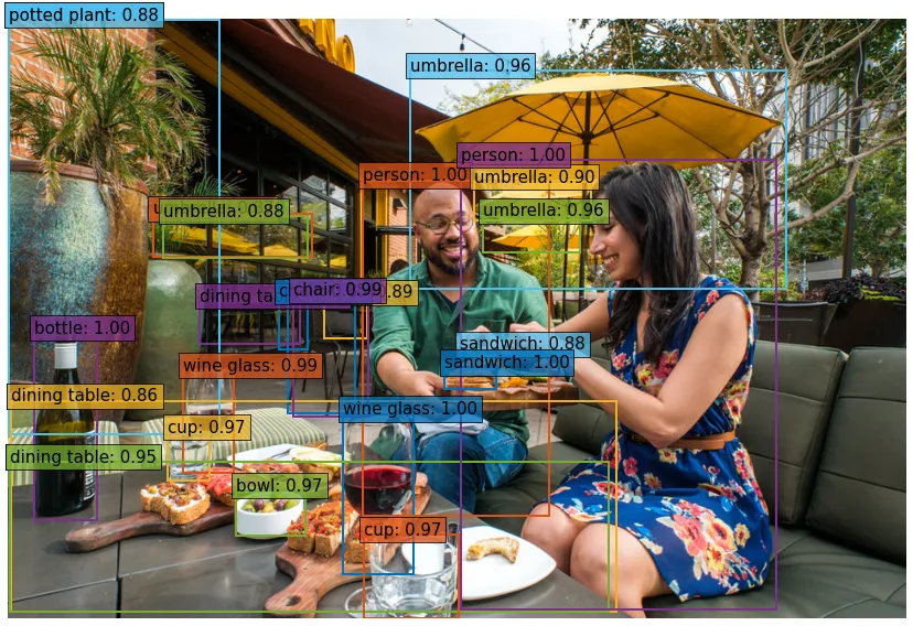
Now that we have our detected objects, we can use a simple function to visualize them
# Plot Predicted Bounding Boxesdef plot_results(pil_img, prob, boxes,labels=True):
    plt.figure(figsize=(16,10))
    plt.imshow(pil_img)
    ax = plt.gca()

    for prob, (x0, y0, x1, y1), color in zip(prob, boxes.tolist(),   COLORS * 100):        ax.add_patch(plt.Rectangle((x0, y0), x1 - x0, y1 - y0,
             fill=False, color=color, linewidth=2))
        cl = prob.argmax()
        text = f'{CLASSES[cl]}: {prob[cl]:0.2f}'
        if labels:
            ax.text(x0, y0, text, fontsize=15,
                bbox=dict(facecolor=color, alpha=0.75))
    plt.axis('off')
    plt.show()
Now we can visualize the results:
plot_results(image, probs, bboxes, labels=True)
Final Thoughts
This post explained some of the details behind the Detection Transformer. Much of the code was inspired by the author’s tutorials which can be found here:
For more information on DETR, see the original author’s github page, and the article introducing the model: