Stock Price Prediction with PyTorch
LSTM and GRU to predict Amazon’s stock prices

Time series problem
Time series forecasting is an intriguing area of Machine Learning that requires attention and can be highly profitable if allied to other complex topics such as stock price prediction. Time series forecasting is the application of a model to predict future values based on previously observed values.
By definition, a time series is a series of data points indexed in time order. This type of problem is important because there is a variety of prediction problems that involve a time component, and finding the data/time relationship is key to the analysis (e.g. weather forecasting and earthquake prediction). However, these problems are neglected sometimes because modeling this time component relationship is not as trivial as it may sound.
Stock market prediction is the act of trying to determine the future value of a company stock. The successful prediction of a stock’s future price could yield a significant profit, and this topic is within the scope of time series problems.
Among the several ways developed over the years to accurately predict the complex and volatile variation of stock prices, neural networks, more specifically RNNs, have shown significant application on the field. Here we are going to build two different models of RNNs — LSTM and GRU — with PyTorch to predict Amazon’s stock market price and compare their performance in terms of time and efficiency.
Recurrent Neural Network (RNN)
A recurrent neural network (RNN) is a type of artificial neural network designed to recognize data’s sequential patterns to predict the following scenarios. This architecture is especially powerful because of its nodes connections, allowing the exhibition of a temporal dynamic behavior. Another important feature of this architecture is the use of feedback loops to process a sequence. Such a characteristic allows information to persist, often described as a memory. This behavior makes RNNs great for Natural Language Processing (NLP) and time series problems. Based on this structure, architectures called Long short-term memory (LSTM), and Gated recurrent units (GRU) were developed.
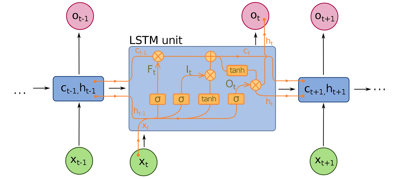
An LSTM unit is composed of a cell, an input gate, an output gate, and a forget gate. The cell remembers values over arbitrary time intervals, and the three gates regulate the flow of information into and out of the cell.
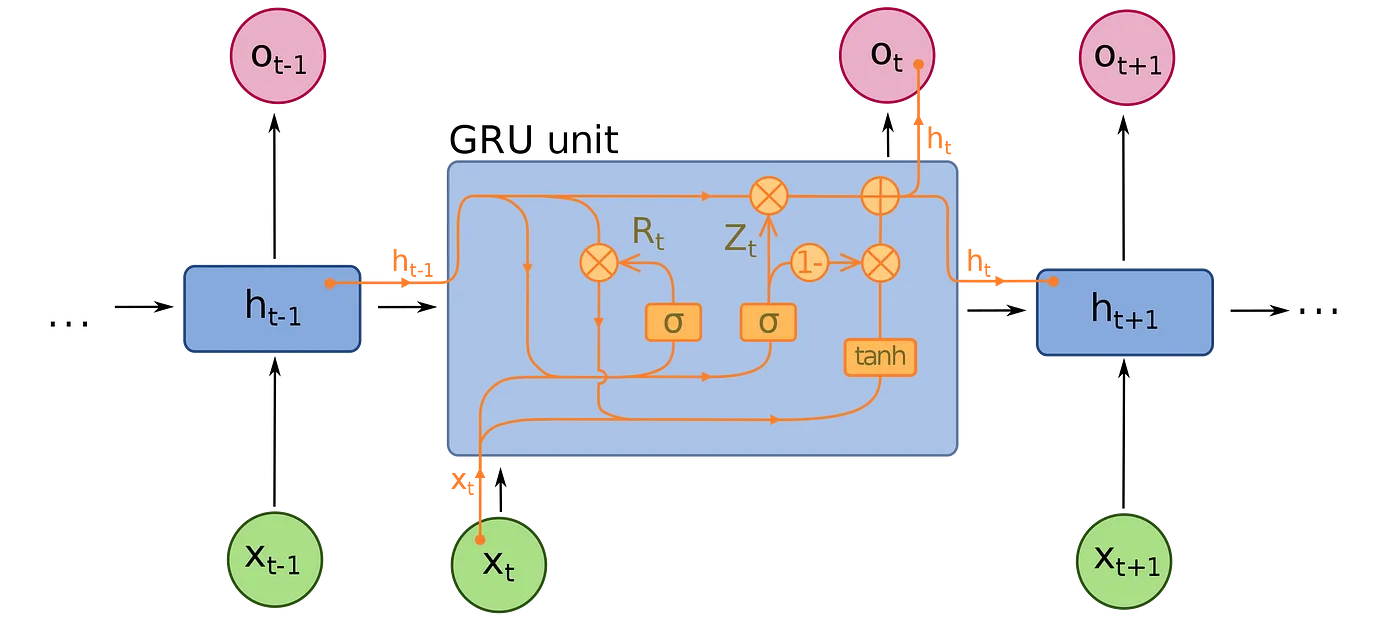
On the other hand, a GRU has fewer parameters than LSTM, lacking an output gate. Both structures can address the “short-term memory” issue plaguing vanilla RNNs and effectively retain long-term dependencies in sequential data.
Although LSTM is currently more popular, the GRU is bound to eventually outshine it due to a superior speed while achieving similar accuracy and effectiveness. We are going to see that we have a similar outcome here, and the GRU model also performs better in this scenario.
Model implementation
The dataset contains historical stock prices (last 12 years) of 29 companies, but I chose the Amazon data because I thought it could be interesting.

We are going to predict the Close price of the stock, and the following is the data behavior over the years.

We slice the data frame to get the column we want and normalize the data.
from sklearn.preprocessing import MinMaxScalerprice = data[['Close']]scaler = MinMaxScaler(feature_range=(-1, 1))
price['Close'] = scaler.fit_transform(price['Close'].values.reshape(-1,1))
Now we split the data into train and test sets. Before doing so, we must define the window width of the analysis. The use of prior time steps to predict the next time step is called the sliding window method.
def split_data(stock, lookback):
    data_raw = stock.to_numpy() # convert to numpy array
    data = []

    # create all possible sequences of length seq_len
    for index in range(len(data_raw) - lookback):
        data.append(data_raw[index: index + lookback])

    data = np.array(data);
    test_set_size = int(np.round(0.2*data.shape[0]));
    train_set_size = data.shape[0] - (test_set_size);

    x_train = data[:train_set_size,:-1,:]
    y_train = data[:train_set_size,-1,:]

    x_test = data[train_set_size:,:-1]
    y_test = data[train_set_size:,-1,:]

    return [x_train, y_train, x_test, y_test]lookback = 20 # choose sequence length
x_train, y_train, x_test, y_test = split_data(price, lookback)
Then we transform them into tensors, which is the basic structure for building a PyTorch model.
import torch
import torch.nn as nnx_train = torch.from_numpy(x_train).type(torch.Tensor)
x_test = torch.from_numpy(x_test).type(torch.Tensor)
y_train_lstm = torch.from_numpy(y_train).type(torch.Tensor)
y_test_lstm = torch.from_numpy(y_test).type(torch.Tensor)
y_train_gru = torch.from_numpy(y_train).type(torch.Tensor)
y_test_gru = torch.from_numpy(y_test).type(torch.Tensor)
We define some common values for both models regarding the layers.
input_dim = 1
hidden_dim = 32
num_layers = 2
output_dim = 1
num_epochs = 100
LSTM
class LSTM(nn.Module):
    def __init__(self, input_dim, hidden_dim, num_layers, output_dim):
        super(LSTM, self).__init__()
        self.hidden_dim = hidden_dim
        self.num_layers = num_layers

        self.lstm = nn.LSTM(input_dim, hidden_dim, num_layers, batch_first=True)
        self.fc = nn.Linear(hidden_dim, output_dim)    def forward(self, x):
        h0 = torch.zeros(self.num_layers, x.size(0), self.hidden_dim).requires_grad_()
        c0 = torch.zeros(self.num_layers, x.size(0), self.hidden_dim).requires_grad_()
        out, (hn, cn) = self.lstm(x, (h0.detach(), c0.detach()))
        out = self.fc(out[:, -1, :])
        return out
We create the model, set the criterion, and the optimiser.
model = LSTM(input_dim=input_dim, hidden_dim=hidden_dim, output_dim=output_dim, num_layers=num_layers)
criterion = torch.nn.MSELoss(reduction='mean')
optimiser = torch.optim.Adam(model.parameters(), lr=0.01)
Finally, we train the model over 100 epochs.
import timehist = np.zeros(num_epochs)
start_time = time.time()
lstm = []for t in range(num_epochs):
    y_train_pred = model(x_train)    loss = criterion(y_train_pred, y_train_lstm)
    print("Epoch ", t, "MSE: ", loss.item())
    hist[t] = loss.item()    optimiser.zero_grad()
    loss.backward()
    optimiser.step()

training_time = time.time()-start_time
print("Training time: {}".format(training_time))

Having finished the training, we can apply the prediction.

The model behaves well with the training set, but it has a poor performance with the test set. The model is probably overfitting, especially taking into consideration that the loss is minimal after the 40th epoch.
GRU
The code for the GRU model implementation is very similar.
class GRU(nn.Module):
    def __init__(self, input_dim, hidden_dim, num_layers, output_dim):
        super(GRU, self).__init__()
        self.hidden_dim = hidden_dim
        self.num_layers = num_layers

        self.gru = nn.GRU(input_dim, hidden_dim, num_layers, batch_first=True)
        self.fc = nn.Linear(hidden_dim, output_dim)

    def forward(self, x):
        h0 = torch.zeros(self.num_layers, x.size(0), self.hidden_dim).requires_grad_()
        out, (hn) = self.gru(x, (h0.detach()))
        out = self.fc(out[:, -1, :])
        return out
Similarly creating the model and setting the parameters.
model = GRU(input_dim=input_dim, hidden_dim=hidden_dim, output_dim=output_dim, num_layers=num_layers)
criterion = torch.nn.MSELoss(reduction='mean')
optimiser = torch.optim.Adam(model.parameters(), lr=0.01)
The training step is exactly the same, and the results we achieve are somehow similar as well.

However, when it comes to the prediction, the GRU model is clearly more accurate in terms of the prediction, as we observe in the following graph.

Conclusion
Both models have good performances in the training phase but stagnate around the 40th epoch, which means that they do not need 100 epochs beforehand defined.
As expected, the GRU neural network outperformed the LSTM in terms of precision because it reached a lower mean square error (in training, and most importantly, in the test set) and in speed, seen that GRU took 5s less finish the training than the LSTM.

Code related questions — https://www.kaggle.com/rodsaldanha/stock-prediction-pytorch