Using Decision Trees and Random Forests to Predict Lending Profitability

This project uses lending data from LendingClub.com to determine if potential customers will successfully pay off a loan after entering a lending agreement. Our main goal will be to compare two models: one created using a single decision tree, the other using a random forest.
Note: This project was covered in a Udemy “Python for Data Science & Machine Learning” course. My code and explanations are shown below. This post is for demonstration purposes only and is not meant to be a tutorial or exhaustive guide.
We’ll start off with the usual analytics workflow — import some relevant libraries, read in the data (from a course-provided CSV file), and do some exploratory data analysis (EDA) to see what exactly we’re working with.
Importing Libraries
import pandas as pd
import numpy as np
import matplotlib.pyplot as plt
import seaborn as sns
%matplotlib inline #this line is for viewing plots in Jupyter
Reading the Data and Viewing the DataFrame
loans = pd.read_csv('loan_data.csv') #reads a CSV into a DataFrame
loans.info()
The .info() call shows us the names of the columns (0–13) and the number of rows (9578), among other things. The most relevant columns that we’ll be checking out today are:
- int.rate: The interest rate of a loan. Borrowers that are deemed “more risky” would be subject to a higher interest rate loan.
- fico: the customers FICO score.
- credit.policy: a 1 if the customer met the lending criteria, and a 0 if not.
- purpose: the purpose of the loan — whether that’s to pay off a credit card, pay student loans, debt consolidation, etc.
- not.fully.paid: our main column of interest that we’ll be trying to predict. We want to see if our use of various machine learning algorithms can help us to predict whether or not someone will pay back their loan based on the given data. This is either a 1 or a 0, 1 meaning the customer did not pay their loan back on time and in full.
The rest of the columns are important to our future models but aren’t necessary to explain here. The main idea is that, based on data for a specific customer (their FICO score, how many days the credit line has been open, the size of each monthly installment, their public records, etc.) we should be able to predict how likely they are to pay their loan off in full.
This has obvious business-driven importance — if our model assigns someone a score of 1 for the not.fully.paid variable, then we may want to re-evaluate our loan agreement with them and find some way to intervene. Correctly identifying (with a reasonable amount of accuracy) those who are likely to default on a loan is a top priority of any loan origination business (or private individual) and could significantly affect the bottom line profitability of the company.
Exploratory Data Analysis
Let’s do some EDA. The following graph compares the FICO scores of two groups — the people who did not meet the lending criteria versus those who did. We’ll utilize some built-in Pandas functionality to overlay two histograms.

The above graph demonstrates the distribution of FICO scores in this study. Though nothing revelational, it shows us that there were more people who passed the lending process than failed it, and that the average FICO score tends to be lower for people who failed.
Next, we’ll use a Seaborn countplot to visualize the various reasons or purposes for taking out a loan, and if that purpose affects the default rate.
plt.figure(figsize=(12,7))
sns.countplot(x = 'purpose', data = loans, hue = 'not.fully.paid', palette = 'pastel')
plt.title('Purposes of Loan Origination')
Debt consolidation appears to be the primary purpose for taking out a loan, and each purpose has a (mostly) similar ratio of success to failure.
Now we’ll use a jointplot to visually confirm what we might expect regarding interests rates and FICO scores — as your FICO score increases, the interest you pay on a loan should be more favorable.
sns.jointplot(x = 'fico', y = 'int.rate', data = loans, color = 'royalblue')
To finish off our EDA, lets see what trends there are when comparing not.fully.paid and credit.policy. We can use an lmplot to fit regression models across conditional subsets of a dataset. It sounds complicated — what we’re really doing is allowing multiple variables to be compared in one figure.
sns.lmplot(x = 'fico', y = 'int.rate', data = loans, col = 'not.fully.paid', hue = 'credit.policy', markers = ['o', 'x'], palette = 'mako')
In this case, we want to see if the relationship between FICO scores and interest rate change at all depending on whether or not the customer paid back their loan. From the above graphs we can see that the trend (indicated by the regression line of best fit) remains largely the same across the split.
Preparing Data For Use With Machine Learning Algorithms
So now we’re ready to get started prepping the data. Before we can fully utilize the scikit-learn ML algos, we need to replace any categorical columns with dummy variables so that each data point is represented numerically rather than with words/strings. Recall the image from when we first checked the DataFrame:
Notice how column 1, purpose, is listed as an “object”— non-numerical. We can use pd.get_dummies() to create a new DataFrame with additional columns, like so:
final_data = pd.get_dummies(data = loans, columns = ['purpose'], drop_first = True)final_data.info()

Now we have 19 columns instead of 14 — the 6 new columns (with the original purpose column removed) each represent one purpose, with a “1” in only one of the last 6 columns to indicate which purpose applies to each customer (see below).

Train-Test Split
The train-test split procedure is used when you want to evaluate the performance of a supervised machine learning algorithm. You split the data into two subsets. The “train” subset will be used to fit the machine learning model, where the “test” subset will be used to, you guessed it, test the performance of the model.
This is an important distinction. You wouldn’t want to train the model and test the model using the same data — that would be cheating, since the model would have already seen the data it’s being asked to predict. More technically, using a train-test split procedure avoids overfitting, where a model has near perfect accuracy when handling training data.
from sklearn.model_selection import train_test_splitX = final_data.drop('not.fully.paid', axis = 1)
y = final_data['not.fully.paid']X_train, X_test, y_train, y_test = train_test_split(X, y, test_size=0.3, random_state=101)
Note that we’ve split our data into two variables, X and y, because the y value is what we’re interested in predicting — in this case, only whether or not the customer has paid back their loan. The X variable should contain everything else in the dataset.
Decision Tree Model

The code behind a decision tree is relatively straightforward. We won’t get in to how the model actually works — you can read all about it in the scikit-learn documentation. Below, we’ll fit the model and then print out a classification report to assess its performance.
from sklearn.tree import DecisionTreeClassifierdtree = DecisionTreeClassifier()
dtree.fit(X_train, y_train)
from sklearn.metrics import classification_report, confusion_matrixpredictions = dtree.predict(X_test)
print(classification_report(y_test, predictions))

We’ll tackle the classification report by looking at the first two columns. Precision is the proportion of predictions in that class that are true. This model accurately predicted 86% of the 0’s and 19% of the 1’s. Remember that our interest is in predicting the 1’s — the people who did not repay their loans. Recall is the ability of the model to correctly identify positive samples. This model correctly identified 24% of the true 1’s in our test data.
Random Forest Model
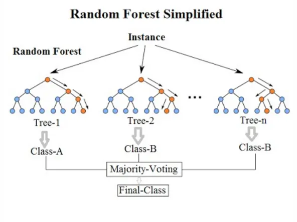
The random forest model creates a combined output of multiple randomly generated decision trees (at the cost of greater training time). As the name implies, the forest is made up of multiple trees. A random forest does not rely on feature importance that can often be a crux of singular decision tree models.
from sklearn.ensemble import RandomForestClassifier
rf = RandomForestClassifier(n_estimators = 600)
rf.fit(X_train,y_train)predictions_rfc = rf.predict(X_test)
print(classification_report(y_test, predictions_rfc))

Comparing the two classification reports, it’s not immediately obvious which model performed “better” than the other. This is where you’ll require an intuitive understanding of the problem, the dataset, and the potential strengths and weakness of each model type. The random forest has a higher overall accuracy, though accuracy as a singular metric can oftentimes be misleading. Note how the random forest has poor recall (only 3%!), meaning it only correctly identified 3% of the people who failed to pay back their loans based on the test data. Ultimately, the model you choose will depend on exactly which parameter you’re trying to optimize for.
This has been a demonstration of decision trees, random forests, and a set of real world data to showcase how machine learning concepts and EDA can be used to extract meaningful insights for businesses.