Using Deep Learning Semantic Segmentation method for Ship detection on Satellite Optical Imagery

Maxence Boels

Published in

The Startup

7 min readOct 26, 2019

A Satellite Remote Sensing Use case

The Competition

A lot of work has been done over the last 10 years to automatically extract objects from satellite images with significative results but no effective operational effects.

Now Airbus is turning to Kagglers to increase the accuracy and speed of automatic ship detection.

Background

Shipping traffic is growing fast. More ships increase the chances of infractions at sea like environmentally devastating ship accidents, piracy, illegal fishing, drug trafficking, and illegal cargo movement. This has compelled many organizations, from environmental protection agencies to insurance companies and national government authorities, to have a closer watch over the open seas.

Data set

The train_ship_segmentations.csv file provides the ground truth (masks of ships) in each image. If there are no ships, the EncodedPixel column is blank.
The sample_submission files contain the images in the test images.

The Data Set and Competition can be found on Kaggle or on the Airbus Sandbox platform.

What is Semantic Segmentation

Let’s first define some crucial concepts to make sure everyone is on the same page.

Image Classification

Let’s start with the simplest, image classification.

Each image corresponds to one and only class from a set of different classes. Thus, here we attribute a specific class to each input image.

We can go further and localize the class object within the image. Here is another cat in case one was not enough.

Object Detection

As I explained above, the challenge in object detection is to surround each class object in an image with the corresponding bounding box. So, the difference with image classification is that each image can have multiple classes instead of one and only. Usually, we add a probability value for each object belonging to a class.

Semantic Segmentation

This technique is what we try to achieve in the Airbus ship detection competitions on Kaggle.

This is a pixel-level classification problem where we want to apply a mask on each class object {Person, Bicycle, Background}. Later, I’ll explain how the evaluate the mask precision on predicted ships in each image regarding the ground truth (real number of ships and their localization on each image).

Instance Segmentation

Finally, instance segmentation is going one step further and is classifying each instance of a class separately. For example, this method could detect 2 cats and 2 dogs in an image but each of the 4 animals has his own segmentation. Whereas, semantic segmentation is not discriminating objects from the same class. For example on the following image (instance segmentation), there are 3 people, technically 3 instances of the class “Person”. But the 3 are classified separately (in a different color).

Now that this is clear for everyone, we can dive into the deep blue ocean and try to detect all ships. Small exercise with the naked eye on the next image.

Ship Semantic Segmentation

Let’s get down to the Machine Learning script

First, import all necessary libraries and create the working directories

import os
import numpy as np # linear algebra
import pandas as pd # data processing, CSV file I/O (e.g. pd.read_csv)
from skimage.io import imread
import matplotlib.pyplot as plt
from skimage.segmentation import mark_boundaries
from skimage.util import montage
import gc; gc.enable() # memory is tight
from skimage.morphology import labelmontage_rgb = lambda x: np.stack([montage(x[:, :, :, i]) for i in range(x.shape[3])], -1)
ship_dir = '../input/airbus-ship-detection'
train_image_dir = os.path.join(ship_dir, 'train_v2')
test_image_dir = os.path.join(ship_dir, 'test_v2')

Then, get some metadata.

masks = pd.read_csv(os.path.join('../input/airbus-ship-detection/',
                                 'train_ship_segmentations_v2.csv'))
print(masks.shape[0], 'masks found')#output
231723 masks found

After that, I can split the data into the training set and validation set.

from sklearn.model_selection import train_test_split
train_ids, valid_ids = train_test_split(unique_img_ids, 
                 test_size = 0.3, 
                 stratify = unique_img_ids['ships'])train_df = pd.merge(masks, train_ids)
valid_df = pd.merge(masks, valid_ids)
print(train_df.shape[0], 'training masks')
print(valid_df.shape[0], 'validation masks')#output
161048 training masks
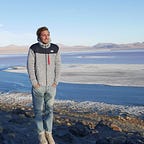
69034 validation maskstrain_df['ships'].hist(bins=np.arange(16)

Since we grouped our data set by imageId and aggregated their binary value no_ships=0 and ships=1. This histogram depicts on the x-axis the number of aggregated ships per imageId. We can observe a majority of images without ships and a normal decreasing distribution of unique imageId with a least one ship.

Histogram: frequency of image with and without ships

Therefore, we need to have a better-balanced training dataset.

Undersample the empty images to get a better-balanced group classes

This code is filtering more the class without ships to create a uniform distribution.

train_df['grouped_ship_count'] = train_df['ships'].map(lambda x: (x+1)//2).clip(0, 7)#floor div // rounds the result down to the nearest whole number
#train_df['grouped_ship_count'].hist()                                                #clip() sets min and max intervals.
def sample_ships(in_df, base_rep_val=1500):
    if in_df['ships'].values[0]==0:
        return in_df.sample(base_rep_val//3) # even more strongly undersample no ships
    else:
        return in_df.sample(base_rep_val, replace=(in_df.shape[0]<base_rep_val))
    
balanced_train_df = train_df.groupby('grouped_ship_count').apply(sample_ships)
balanced_train_df['ships'].hist(bins=np.arange(16)) #with 10 bins

Image processing, filtering, and masks

Sample data, generated masks, and the ground truth

U-Net Model Design

The architecture looks like a ‘U’ which justifies its name. This architecture consists of three sections: The contraction, The bottleneck, and the expansion section. But the heart of this architecture lies in the expansion section. This action would ensure that the features that are learned while contracting the image will be used to reconstruct it.

from keras import models, layers
# Build U-Net model
def upsample_conv(filters, kernel_size, strides, padding):
    return layers.Conv2DTranspose(filters, kernel_size, strides=strides, padding=padding)
def upsample_simple(filters, kernel_size, strides, padding):
    return layers.UpSampling2D(strides)if UPSAMPLE_MODE=='DECONV':
    upsample=upsample_conv
else:
    upsample=upsample_simple
    
input_img = layers.Input(t_x.shape[1:], name = 'RGB_Input')
pp_in_layer = input_img
if NET_SCALING is not None:
    pp_in_layer = layers.AvgPool2D(NET_SCALING)(pp_in_layer)
    
pp_in_layer = layers.GaussianNoise(GAUSSIAN_NOISE)(pp_in_layer)
pp_in_layer = layers.BatchNormalization()(pp_in_layer)c1 = layers.Conv2D(8, (3, 3), activation='relu', padding='same') (pp_in_layer)
c1 = layers.Conv2D(8, (3, 3), activation='relu', padding='same') (c1)          #Going Down
p1 = layers.MaxPooling2D((2, 2)) (c1) #2x2 kernelc2 = layers.Conv2D(16, (3, 3), activation='relu', padding='same') (p1)
c2 = layers.Conv2D(16, (3, 3), activation='relu', padding='same') (c2)
p2 = layers.MaxPooling2D((2, 2)) (c2)c3 = layers.Conv2D(32, (3, 3), activation='relu', padding='same') (p2)
c3 = layers.Conv2D(32, (3, 3), activation='relu', padding='same') (c3)
p3 = layers.MaxPooling2D((2, 2)) (c3)c4 = layers.Conv2D(64, (3, 3), activation='relu', padding='same') (p3)
c4 = layers.Conv2D(64, (3, 3), activation='relu', padding='same') (c4)
p4 = layers.MaxPooling2D(pool_size=(2, 2)) (c4)c5 = layers.Conv2D(128, (3, 3), activation='relu', padding='same') (p4)       #Bottle Neck
c5 = layers.Conv2D(128, (3, 3), activation='relu', padding='same') (c5)u6 = upsample(64, (2, 2), strides=(2, 2), padding='same') (c5)                 #Going Up
u6 = layers.concatenate([u6, c4])
c6 = layers.Conv2D(64, (3, 3), activation='relu', padding='same') (u6)
c6 = layers.Conv2D(64, (3, 3), activation='relu', padding='same') (c6)u7 = upsample(32, (2, 2), strides=(2, 2), padding='same') (c6)
u7 = layers.concatenate([u7, c3])
c7 = layers.Conv2D(32, (3, 3), activation='relu', padding='same') (u7)
c7 = layers.Conv2D(32, (3, 3), activation='relu', padding='same') (c7)u8 = upsample(16, (2, 2), strides=(2, 2), padding='same') (c7)
u8 = layers.concatenate([u8, c2])
c8 = layers.Conv2D(16, (3, 3), activation='relu', padding='same') (u8)
c8 = layers.Conv2D(16, (3, 3), activation='relu', padding='same') (c8)u9 = upsample(8, (2, 2), strides=(2, 2), padding='same') (c8)
u9 = layers.concatenate([u9, c1], axis=3)
c9 = layers.Conv2D(8, (3, 3), activation='relu', padding='same') (u9)
c9 = layers.Conv2D(8, (3, 3), activation='relu', padding='same') (c9)d = layers.Conv2D(1, (1, 1), activation='sigmoid') (c9)
d = layers.Cropping2D((EDGE_CROP, EDGE_CROP))(d)
d = layers.ZeroPadding2D((EDGE_CROP, EDGE_CROP))(d)
if NET_SCALING is not None:
    d = layers.UpSampling2D(NET_SCALING)(d)seg_model = models.Model(inputs=[input_img], outputs=[d])
seg_model.summary()

Model Fitting

Result evaluation

Due to the very slow runtime until the end of the submission. I was limited in the time I could spend on this project. I decided to move forward even though results could be enhanced. There are so many exciting and challenging Satellite Imagery projects to learn from that I could not resist moving on to another project.

Conclusion

This project is a great one to start with and become familiar with Satellite Imagery in machine learning. I hope this article was informative regarding this field and has tickled your curiosity in order to read more about such projects and make you jump into Kaggle competitions (which is the best place to learn from, with practical exercises on real business cases).

I will be writing more about Computer Vision and Machine Learning and especially in the Earth Observation sector. So follow me if you share this interest.