SpaceNet 6: A First Look at Model Performance

Preface: SpaceNet LLC is a nonprofit organization dedicated to accelerating open source, artificial intelligence applied research for geospatial applications, specifically foundational mapping (i.e., building footprint & road network detection). SpaceNet is run in collaboration by co-founder and managing partner, CosmiQ Works, co-founder and co-chair, Maxar Technologies, and our partners including Intel AI, Amazon Web Services (AWS), Capella Space, Topcoder, IEEE GRSS, the National Geospatial-Intelligence Agency and Planet.
Introduction
In this blog we will begin to explore how some of the complexities of Synthetic Aperture Radar (SAR) affected the performance of the winning SpaceNet 6 algorithms. SAR sensors are unique as data is generated by having the sensor actively illuminate the ground rather than utilizing the light from the sun as with optical images. This means that when we look at a SAR image the brightness of each pixel depends on the amount of energy the SAR sensor transmits and receives back at the sensor (known as backscatter). The amount of backscatter received is dictated by the material properties, physical shapes, and the angle from which objects on the ground are viewed. This also means that SAR sensors cannot detect color, but rather the types of backscatter the SAR sensor is receiving. The SAR data in SpaceNet 6 is also captured from an average off-nadir perspective of ~35°. Such off-nadir perspectives, combined with the active sensing of SAR, leads to two further challenges: SAR layover and building occlusion. If you’re interested in understanding more about how SAR works we recommend you read out primer blogs (SAR 101 and SAR 201) on this topic.
In summary, this blog will examine:
- How does building height and size affect model performance?
- How do models trained on optical data compare to the ones trained on SAR in Rotterdam?
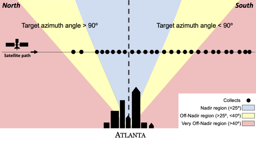
- Drawing from the lessons learned in SpaceNet 4: What is the affect of look angle on model performance?
Building Height and Size
Our first look at some of predictions derived from the winning SpaceNet 6 algorithms explore two aspects of the building footprint dataset: building height and size. We extract the height of each building by using the associated LiDAR height estimates in meters attached to the 3DBAG dataset and extract the size of each building by measuring each footprints total area in meters². We then average the recall scores across 50 different bins of building size or height. Remember that recall is simply the ratio of the number of buildings correctly identified. The lower the recall, the more buildings are missed by the model, the higher — the fewer.


In our imagery in the figure above we can see two of the tallest buildings in Rotterdam: the New Orleans (~158m) and the Montevideo (~140m). On the left image we can see how these tall buildings can cause the unique SAR phenomenon of layover — the buildings stretch out over the water toward the south. In this setting, the SAR sensor is capturing data from the south with its sensor pointing north. The radar signal reaches the top of the building first, then the base, causing this layover effect. On the right image, we can see how these structures appear in our optical data shot from ~17° off-nadir.
The center plot visualizes how performance changes based upon building height. Performance from the winners model (zbigniewwojna — blue) begins to gradually decline as height increases. Similar trends are observed from MaksimovKA — orange (2nd) and SatShipAI — green (3rd), however this trend is certainly noisier and we see some interesting peaks in performance around 60 meters in height. More data and research is obviously required to validate these findings, although this downward trend does suggest that some of the distortions from the SAR data can cause complications for computer vision algorithms.


In this next figure, on the rightmost image, we can see a suburban landscape with many tiny houses and some obstructing forest cover. We can see that color could be particularly helpful for pulling out these tiny features, although this would likely still be quite challenging. In the leftmost image, we can see this same landscape in our SAR data. Although the image on the left has some color, this is actually a construct of visualizing three polarizations (that measure different types of backscatter) via the RGB channels. Furthermore, the oblique look angle of the SAR data causes more occlusions from the trees. Overall this produces we have a very textured surface and one of the most challenging images in the dataset. Consequently, only one building is actually detected in this full tile by the winning algorithm — situated in the lower left corner.
The center plot reinforces these findings and shows that each of the top-3 models struggled to correctly identify the tiny structures that were prevalent within the dataset. Any structure smaller than 40 meters² was impossible to identify. You can also see in this plot that the winning algorithm outperforms the others in structures between 100 to 1000 m². These small performance differences proved to be the critical difference in determining the winner of the challenge. Larger structures are certainly much easier with performance for the top-3 algorithms rising gradually until building area reaches about 1000 meters².
A Comparison: Optical Versus SAR
Although the above findings are informative, we were also interested in how well the winning model would have done if it was trained and tested on optical imagery. The winners didn’t have this option as only SAR data was included in the testing datasets. However, SpaceNet has these datasets and as such we are able to train and score the algorithms on only optical imagery. In this case we replace the SAR data with pan-sharpened RGB+NIR imagery as our model input. As both data are four-channels we can easily swap them out in the network.
We make no changes to the winners algorithm besides this change in data. As such, we caveat this experiment by noting that the winners algorithm was tuned specifically for the SpaceNet 6 SAR data. Performance for optical imagery likely could be improved with some different pre-processing steps and augmentations throughout the training process. Another caveat is again the difference in look angles. SpaceNet 4 showed us that performance dips significantly as look angle becomes more oblique. For a true comparison it would be best to perform these test with optical data captured from an equivalent off-nadir perspective as well. That being said, we can estimate how much performance would decline using the findings of SpaceNet 4 to guide us, which we will discuss later.


As expected from these results, optical data does indeed outperform SAR data. This shouldn’t be surprising — computer vision algorithms are specifically designed to work with such data. This is one of the reasons why we were motivated to create the SpaceNet 6 dataset and challenge. We believe that openly releasing very high resolution SAR data can foster innovation and research to continue to improve upon these results. The overall SpaceNet score (F1 with an IOU threshold of 0.5) achieved by the optical model is a 0.69, a ~63% increase over the SAR only model which scored a 0.42.
Examining the plot on the left we can see the performance differences based upon building height. The downward trend is evident for SAR data as buildings increase in height, however for optical data the performance is much noisier. Overall, building height is likely not as strongly correlated with model performance when using optical data; particularly from a mostly on-nadir perspective. The most interesting comparisons are for structures taller than 60 meters where we can see the optical performance peaks and diverges from the SAR performance. A larger sample of buildings would help to validate these results further.
The plot on the right shows that building size is also quite important for optical imagery. With optical data we are able to detect some smaller structures with performance peaking around 300 meters² and stabilizing. Performance of the optical model is certainly less noisy versus our height plot, indicating that building size is much more likely to be correlated with model performance than building height is.
A Comparison: SpaceNet 4
The SpaceNet 4 dataset over Atlanta was extremely valuable as it captured the same area from 27 different look angles over just a few minutes of time. The on-nadir spatial resolution of this data also matches the Rotterdam collect (0.5m). As such we can do a few direct comparisons and investigate the performance differences based on modality and off-nadir angle.

Overall these results are interesting and we can see the on-nadir optical performance is a bit worse vs. SpaceNet 4. There are likely several reasons for this, but notably:
- The SpaceNet 4 dataset is larger (127,000 vs. 48,000 building footprints)
- Cannab trained his model on all 27 look-angles at once meaning there are many perspectives of the same areas that a model uses to learn
- Zbigniewwojnas model is optimized for the SAR data, not the optical data.
The final interesting aspect of this analysis is the performance difference of the SAR versus the optical data when both are captured at ~35° off-nadir. We note that there are certainly a number of confounding factors here that can cloud our understanding of these results such as: geographic differences, a coarser spatial resolution of the optical data at oblique look angles, and the fact that we are looking at two very different domains (SAR vs Optical). However, we can hypothesize a bit: These results may indicate that if the SAR data was a bit more on-nadir, performance could be slightly improved as there would be fewer occlusions and layover effects would be less severe. Overall, these results seem to indicate that more SAR specific methods and research is required to continue further unlock the potential of SAR for foundational mapping applications.
Coming Up
Over the next weeks we will continue our analysis and begin our software releases. Lookout for posts on:
- Time Series Investigation: Does combining a deep stack of model predictions help to improve model performance?
- Colorization: Can we run a colorization pre-processing step on the SAR data to inject some color, thus improving model performance?
- Solaris Code Update: A pre-processing pipeline and codebase for working with SAR data.
- Top 5 Algorithm Release: We open source the SpaceNet 6 prize winning algorithms
