Delve into Sequences: Understanding the Power of Sequential Data in Machine Learning

Use sequential data properly in your next data science task

In common machine learning tasks, the data is assumed to be identically and independently distributed (i.i.d.). However, when dealing with changes in the distribution of the underlying data-generating process, or working with data with temporal dependence, this i.i.d. assumption breaks.

➜ Pro tip: If you like to learn faster and run (or download) this project in Jupyter Notebook for free, visit CognitiveClass.ai.

Practitioners and data scientists should be able to model such data by drawing from various tools for sequential data analysis. In this project, we introduce forms of sequential data, and basic concepts needed to understand the components of a time series.

Machine Learning for Sequential Data

Background

In machine learning, data is often assumed to be i.i.d., meaning each sample is independent of the others. However, sequential data violates this assumption since samples rely on past information. Examples include weather and financial time series. Classic methods exist to study time series data before Recurrent Neural Networks (RNNs) were developed to better model sequential data.

The i.i.d. Assumption

In this project, we will be dealing with data that, rather than being drawn i.i.d., from some joint distribution P(x, y), actually consists of sequences of (x, y)$ pairs that show some sequential correlation. This means that values close to the x and y values are likely to be related to and/or dependent on each other.

So when the points in the data set are dependent on the other points in the data set, the data is termed sequential.

The sequential supervised learning problem can be formulated as follows:

Let’s

be a set of N training examples. In a part-of-speech tagging task, one $(x_i, y_i)$ pair might consist of x_i = do you want fries and y_i = verb pronoun verb-noun. We aim to build a model, h, that predicts the next label sequence, y = h(x), given an input sequence, x. Here the task is to predict the t+1st element of the sequence (y_1,…,yt).

Let us walk through an example to highlight the issues when working with non-i.i.d. data. We will be using financial quotations from various energy companies.

Data

We provide a zip file including the stock prices of a few companies.

link to download the data:
"https://cf-courses-data.s3.us.cloud-object-storage.appdomain.cloud/IBMDeveloperSkillsNetwork-ML311-Coursera/datasets/financial-data.zip"

import pandas as pd

symbols = {"TOT": "Total", "XOM": "Exxon", "CVX": "Chevron",
           "COP": "ConocoPhillips", "VLO": "Valero Energy"}
template_name = ("./financial-data/{}.csv")

quotes = {}
for symbol in symbols:
    data = pd.read_csv(
        template_name.format(symbol), index_col=0, parse_dates=True
    )
    quotes[symbols[symbol]] = data["open"]
quotes = pd.DataFrame(quotes)
quotes .head()

Let us plot a few financial quotations.

import matplotlib.pyplot as plt

quotes.plot()
plt.ylabel("Quote value")
plt.legend(bbox_to_anchor=(1.05, 0.8), loc="upper left")
_ = plt.title("Stock values over time")

We want to predict the quotation of Chevron using all other energy companies’ quotes. We will use the decision tree regressor that is expected to overfit and thus not generalize to unseen data. We will start off by splitting our data into a testing and training set.

data, target = quotes.drop(columns=["Chevron"]), quotes["Chevron"]
data_train, data_test, target_train, target_test = train_test_split(
    data, target, shuffle=True, random_state=0)

Let’s now define our model, and we apply a cross-validation strategy, to check the generalization performance of our model.

regressor = DecisionTreeRegressor()
cv = ShuffleSplit(random_state=0)
regressor.fit(data_train, target_train)
target_predicted = regressor.predict(data_test)
# Affect the index of `target_predicted` to ease the plotting
target_predicted = pd.Series(target_predicted, index=target_test.index)
target_predicted 

Now we perform the evaluation.

from sklearn.metrics import r2_score

test_score = r2_score(target_test, target_predicted)
print(f"The R2 on this single split is: {test_score:.2f}")

#outcome is: The R2 on this single split is: 0.82 

We get outstanding generalization performance in terms of 𝑅^2. Let’s plot the predictions against the ground truth.

target_train.plot(label="Training")
target_test.plot(label="Testing")
target_predicted.plot(label="Prediction")

plt.ylabel("Quote value")
plt.legend(bbox_to_anchor=(1.05, 0.8), loc="upper left")
_ = plt.title("Model predictions using a ShuffleSplit strategy")

The results are surprisingly very good, as we had originally expected the model to overfit and not generalize on unseen test sets. Let us now investigate why this is the case.

We used a cross-validation method that shuffles data and splits. We will simplify this procedure by not shuffling our data and plotting the results obtained.

data_train, data_test, target_train, target_test = train_test_split(
    data, target, shuffle=False, random_state=0,
)
regressor.fit(data_train, target_train)
target_predicted = regressor.predict(data_test)
target_predicted = pd.Series(target_predicted, index=target_test.index)

test_score = r2_score(target_test, target_predicted)
print(f"The R2 on this single split is: {test_score:.2f}")
# The R2 on this single split is: -2.21

let's plot the model prediction without shuffling

Now we see that our model performs worse than just predicting the mean of the target. Why is that?

In time series datasets, subsequent samples are dependent on previous samples, violating the i.i.d. assumption. Models can predict well due to data leakage or memorization of the training data.

Forms of Sequential Data

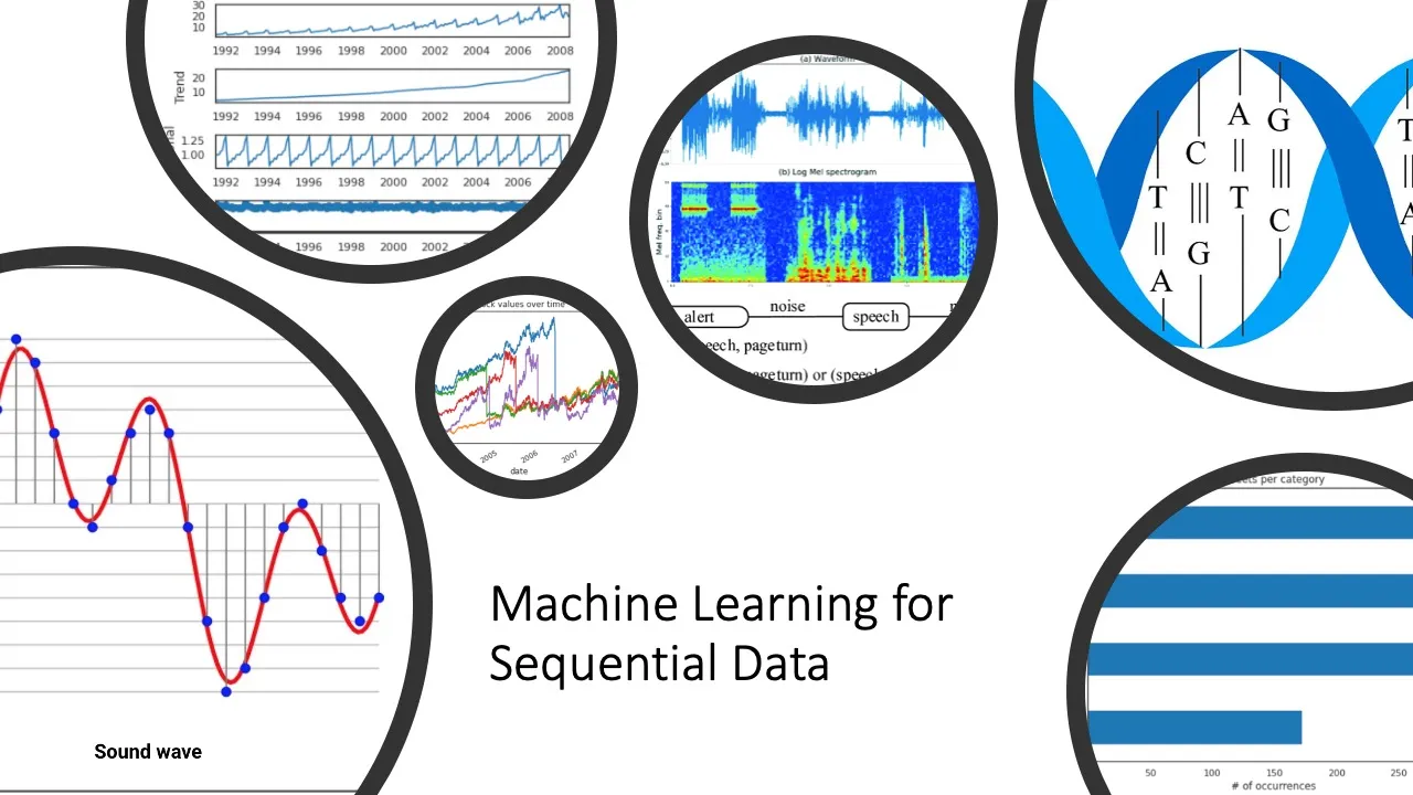
Sequential data contains elements that are ordered into sequences. For example, time series (like stock values or sensor measurements), gene sequences (𝐶,𝐺,𝐴,𝑇), speech, text (𝑎,…, 𝑧, 0, …, 9), video clips, and musical notes, and so on.

To summarize, sequential data has some temporal coherence and can be of arbitrary lengths. A lot of tasks can be modeled from these types of data. For example:

• text classification, such as spam email or not
• language translation, such as French to English
• time-series forecasting, such as stock prices prediction

Let us look at a few common sequential data sets, and understand pre-processing techniques associated with each.

Working with time-series data

Time series are special types of sequences that consist of random variables indexed by time. In particular, the random variables can be dependent and their distribution might change over time, so time-series also violate the i.i.d. assumption

Time-series decomposition

Time series data can exhibit various patterns, and it is often helpful to split a time series into several components, each representing an underlying pattern category. These include trends, seasonality, and cycles, which we will now explain using examples.

• trend: A trend is observed when there is an increasing or decreasing slope observed in the time series. In the following time series, we see an increasing pattern.

trend = pd.read_csv('https://cf-courses-data.s3.us.cloud-object-storage.appdomain.cloud/IBMDeveloperSkillsNetwork-ML311-Coursera/labs/Module4/L1/guinearice.csv', parse_dates=['date'], index_col='date')
plt.plot(trend.values)

• seasonality: Seasonality represents a distinct repeated pattern observed between regular intervals due to seasonal factors, like a month of the year, the day of the month, weekdays or even times of the day, festivals, and so on.

seasonality = pd.read_csv('https://cf-courses-data.s3.us.cloud-object-storage.appdomain.cloud/IBMDeveloperSkillsNetwork-ML311-Coursera/labs/Module4/L1/sunspotarea.csv', parse_dates=['date'], index_col='date')
plt.plot(seasonality.value)

A time series can have both trend and seasonality, for example:

seasonality_trend = pd.read_csv('https://cf-courses-data.s3.us.cloud-object-storage.appdomain.cloud/IBMDeveloperSkillsNetwork-ML311-Coursera/labs/Module4/L1/AirPassengers.csv', parse_dates=['date'], index_col='date')
plt.plot(seasonality_trend.value)

• cyclic: Cyclicity is similar to seasonality, but it happens when the rise and fall pattern in the series does not happen in fixed calendar-based intervals, that is, if the patterns are not of fixed calendar-based frequencies, then the pattern is cyclic.

A time series can be modeled as an additive or multiplicative, wherein each observation in the series can be expressed as either a sum or a product of the components.

Additive time series

𝑉𝑎𝑙𝑢𝑒(𝑡)=𝐵𝑎𝑠𝑒𝐿𝑒𝑣𝑒𝑙(𝑡)+𝑇𝑟𝑒𝑛𝑑(𝑡)+𝑆𝑒𝑎𝑠𝑜𝑛𝑎𝑙𝑖𝑡𝑦(𝑡)+𝐸𝑟𝑟𝑜𝑟(𝑡)

Multiplicative Time Series

𝑉𝑎𝑙𝑢𝑒(𝑡)=𝐵𝑎𝑠𝑒𝐿𝑒𝑣𝑒𝑙(𝑡)𝑥𝑇𝑟𝑒𝑛𝑑(𝑡)𝑥𝑆𝑒𝑎𝑠𝑜𝑛𝑎𝑙𝑖𝑡𝑦(𝑡)𝑥𝐸𝑟𝑟𝑜𝑟(𝑡)

We can use functions like seasonal_decompose from the python package, statsmodel, to decompose our time-series into the trend, seasonality, and residual components.

# Import Data
df = pd.read_csv('https://cf-courses-data.s3.us.cloud-object-storage.appdomain.cloud/IBMDeveloperSkillsNetwork-ML311-Coursera/labs/Module4/L1/a10.csv', parse_dates=['date'], index_col='date')
plt.plot(df.value)

Let us start by performing additive decomposition. Note that by using extrapolate_trend = 'freq', we impute missing values at the beginning of the time series.

# Additive Decomposition
result_add = seasonal_decompose(df['value'], model='additive', extrapolate_trend='freq')

# Plot
result_add.plot()

Now, similarly, we can try performing multiplicative decomposition:

# Multiplicative Decomposition 
result_mul = seasonal_decompose(df['value'], model='multiplicative', extrapolate_trend='freq')

#Plot
result_mul.plot()

In this particular case, we see that with additive decomposition, some pattern is still left over, while with multiplicative decomposition, the result looks quite random, which is what we want.

So how do we detrend our time series? One way would be to subtract the trend component obtained from the time series decomposition we saw earlier.

detrended = df.value.values - result_mul.trend
plt.plot(detrended)
plt.title('Drug Sales detrended by subtracting the trend component', fontsize=16)

Similarly, we can remove the seasonality component:

deseasonalized = df.value.values / result_mul.seasonal

# Plot
plt.plot(deseasonalized)

Time-series imputation

Earlier, we briefly mentioned imputing missing values in a time-series. Sometimes, your time series will have missing dates/times. That means the data was not captured or unavailable for those periods.

Depending on the nature of the series, we can try multiple approaches for imputation:

• Forward
• Backward Fill
• Linear Interpolation, etc.

Let us start by parsing the data frame indices as dates.

df = pd.read_csv('https://cf-courses-data.s3.us.cloud-object-storage.appdomain.cloud/IBMDeveloperSkillsNetwork-ML311-Coursera/labs/Module4/L1/a10.csv', parse_dates=['date'], index_col='date')

• Forward Imputation

from scipy.interpolate import interp1d
from sklearn.metrics import mean_squared_error

df_ffill = df.ffill()
# Print the MSE between imputed value and ground truth
error = np.round(mean_squared_error(df['value'], df_ffill['value']), 2)
df_ffill['value'].plot(title='Forward Fill (MSE: ' + str(error) +")", label='Forward Fill', style=".-")

• Backward Imputation

df_bfill = df.bfill()
error = np.round(mean_squared_error(df['value'], df_bfill['value']), 2)
df_bfill['value'].plot(title="Backward Fill (MSE: " + str(error) +")", label='Back Fill', color='firebrick', style=".-")

• Linear Interpolation

df['rownum'] = np.arange(df.shape[0])
df_nona = df.dropna(subset = ['value'])
f = interp1d(df_nona['rownum'], df_nona['value'])
df['linear_fill'] = f(df['rownum'])
error = np.round(mean_squared_error(df['value'], df['linear_fill']), 2)
df['linear_fill'].plot(title="Linear Fill (MSE: " + str(error) +")",label='Cubic Fill', color='green', style=".-")

Time-series decomposition and imputation are common pre-processing steps used when working on time-series prediction or forecasting tasks.

More practices

Sequential data is ordered in a specific sequence or time series, and can include text, audio signals, and genetic sequences. Machine learning models can be trained on labeled datasets to predict sentiment in text, audio clipping in audio signals, and gene classification in genetic sequences.

Practice projects are available for further practice👇🏻.

Machine Learning for Sequential Data

Thanks for reading!

You can follow me on Medium or LinkedIn and stay tuned for more articles on Data Science, Machine Learning, and AI.

If you are interested in my project, here is my IBM skills network profile:

Sina Nazeri