Machine learning and Mathematics
Mathematical understanding of Gaussian Process
Detailed explanation of mathematical background of Gaussian process with necessary concepts and visualization
Gaussian process is beneficial, especially when we have a small amount of data. When I worked as a data scientist in the manufacturing industry, our team used this algorithm to reveal which experiment conditions we should conduct next. However, this algorithm is less popular than other algorithms. In this blog, I will explain the mathematical background of Gaussian process [1] with visualization and Python implementation.
Table of Contents
1. Preliminary: Multivariate Gaussian distribution
The multivariate Gaussian distribution is one of the necessary concepts to understand the Gaussian process. Let’s quickly recap it. You can skip this section if you are familiar with the multivariate Gaussian distribution.
The multivariate Gaussian distribution is the joint probability of Gaussian distribution that has more than two dimensions. The multivariate Gaussian distribution has the probability density function below.

x is the input data that has D × 1 dimensions, μ is the mean vector that has the same dimension with x and Σ is the covariance matrix that has D × D dimensions.
The multivariate Gaussian distribution has important features below.
- Marginal distribution of the multivariate Gaussian distribution still follows the Gaussian distribution
- Conditional distribution of the multivariate Gaussian distribution still follows the Gaussian distribution
Let’s check those concepts with visualization. We assume the D-dimensional data follows the Gaussian distribution.
For feature 1, when we divide the input data dimension D into the first L and the other D-L=M dimensions, we can describe the Gaussian distribution as follows.

Then, when we marginalize the distribution with regard to x₂, the probability distribution of x₁ can be written as:

Based on the formula (1), we can cancel other variables when marginalizing them. The graph shows the two-dimensional Gaussian distribution case. As you can see, the marginalized distribution maps to each axis; its form is the Gaussian distribution. Intuitively, the distribution of the cross-section still follows the Gaussian distribution when we cut the multivariate Gaussian distribution according to one axis. You can see the reference [2] for the detailed derivation.
For feature 2, we use the same D-dimensional multivariate Gaussian distribution and two-divided input data x₁ and x₂. The conditional probability of multivariate Gaussian distribution can be written as:

The figure shows the two-dimensional Gaussian distribution (contour line) and conditional Gaussian distributions (dotted lines). The shape of the Gaussian distribution is different in each condition. You can see the reference [2] for the detailed derivation.
1. Linear regression model and the curse of dimensionality
Before diving into the Gaussian process, I want to clarify the linear regression model and its disadvantage or the curse of dimensionality. The Gaussian process is closely related to this concept and can overcome its disadvantages. You can skip this chapter if it rings a bell.
Let’s recap the linear regression model. The linear regression model can flexibly express the data using the basis functions 𝝓(x).

For a basis function, we can use a non-linear function, such as a polynomial term or a cosine function. Thus, the linear regression model can grasp the non-linear relationship by applying non-linear basis functions to x. The following graph shows an example case when we use radial basis functions.

As you can see, it can grasp complex data structures. We still call it a linear regression model because this equation still satisfies the linear relationship from the parameter w point of view. You can check that parameters don’t have non-linear expressions.
We can also derive the parameters in the same way as the multiple linear regression. The following equations are the matrix and linear algebra form of the linear regression model. We assume N data points and p+1 parameters.


Note that the matrix 𝚽 values become the constant after we apply basis functions to each input data. Isn’t it similar to the multiple linear regression? Actually, the analytical derivations of parameters are the same.

There is a pitfall that the linear regression model assumes one independent variable in formula (4). So, when the number of input data dimensions increases, the number of parameters increases exponentially. If we add the number of basis functions, we can get the model’s flexibility, but the computation amount increases unrealistically. This problem is called the curse of dimensionality. Is there any method to improve the model flexibility without increasing the computation amount? Yes, we apply the Gaussian process theorem. Let’s go to the next section and see what the Gaussian process is.
3. Mathematical background of Gaussian Process
We have seen that the linear regression model has a problem with the curse of dimensionality when the number of parameters increases. The solution to this problem is to take an expectation of the parameters and create a situation where parameters are not necessary to compute. What does it mean? Remember, the linear regression model formula is below.
Now, when we assume the parameter w follows the Gaussian distribution, the output y will follow the Gaussian distribution because the matrix 𝚽 is just constant value matrix. We assume the parameter follows the Gaussian distribution below:

Based on it, we can calculate the output distribution’s parameters as follows:


As you can see, we can cancel out the parameter calculation by taking its expectation. Thus, even though we have infinite parameters, they don’t affect the calculation. This relationship between x and y follows the Gaussian process. The Gaussian process definition is:

Intuitively, the Gaussian process is the multivariate Gaussian distribution with an infinite number of parameters. The formula (7) refers to the marginal Gaussian distribution from the Gaussian process by given data. It derives from the feature that the marginal multivariate Gaussian distribution still follows the Gaussian distribution. So, by making good use of Gaussian processes, the model can be constructed while considering parameters of infinite dimension.
Here is another problem, how do we choose the matrix 𝚽? When we focus on the covariance matrix part of the above formula and set it as K, each element can be written as:

According to the formula (9), each element of the covariance matrix is the constant multiple of the inner product of 𝟇(xᵢ) and 𝟇(xⱼ). Since the inner product is analogous to cosine similarity, the value of formula(9) becomes larger values when xᵢ and xⱼ are similar.
To satisfy the features of the covariance matrix that are symmetric and positive-definite and have an inverse matrix, we need to choose 𝟇(x) appropriately. To fulfill them, we utilize the kernel function for 𝟇(x).

One benefit of using the kernel function is that we can get the inner product of 𝟇(x) through the kernel function without explicitly calculating 𝟇(x). This technique is called the kernel trick. You can check this excellent blog [3] for a detailed explanation of the kernel tricks. The most used kernel functions are shown below.
- Gaussian kernel

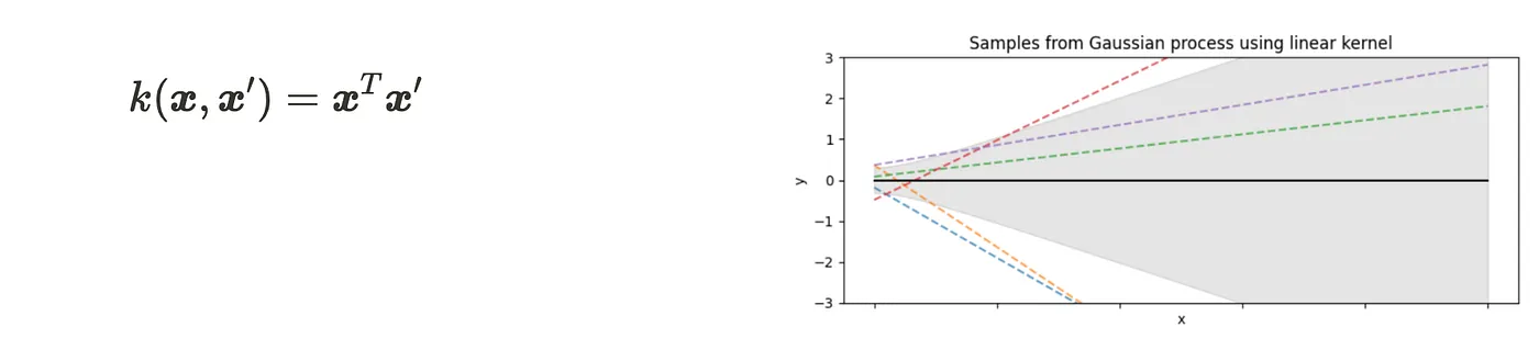
- Linear kernel
- Periodic kernel
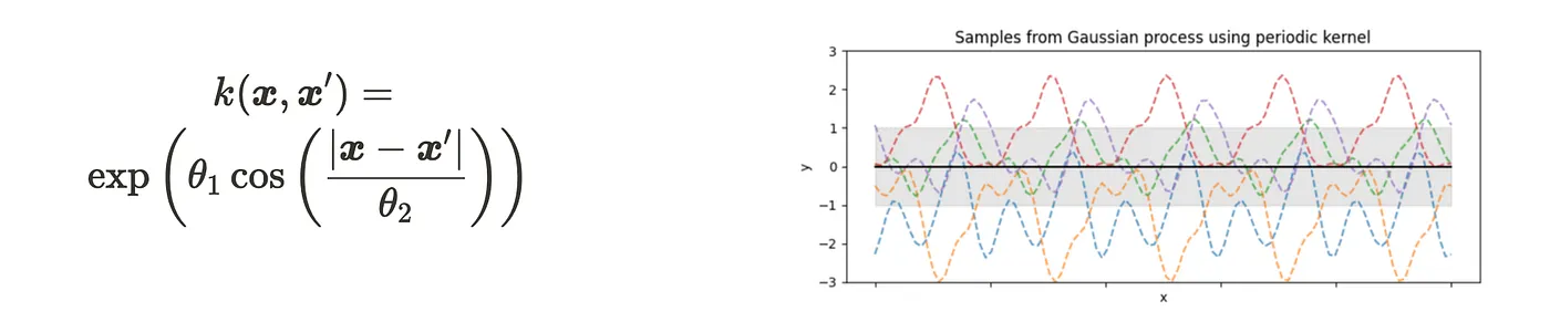
The visualizations show the sampling one-dimensional Gaussian process using each kernel. You can see the features of kernels.
Now, let’s recap the Gaussian process. Using the kernel function, we can rewrite the definition as:

When each element of f follows the Gaussian process, which means the infinite Gaussian distribution, the joint probability of f follows the multivariate Gaussian distribution.
In the next section, we will discuss the application of the Gaussian process, or Gaussian process regression model.
4. The application of the Gaussian process: Gaussian process regression
In the final section, we apply the Gaussian process to regression. We will see the topics below.
- How to fit & inference the Gaussian process model
- Example: Gaussian process model for one-dimensional data
- Example : Gaussian process model for multiple dimensional data
How to fit and inference the Gaussian process model
Let us have N input data x and corresponding outputs y.

For simplicity, we apply normalization to the input data x for preprocessing, which means the mean of x is 0. If we have the following relationship between x and y, and f follows the Gaussian process.

Thus, the output y follows the following multivariate Gaussian distribution.

For fitting, we just calculate the covariance matrix through the kernel function, and the parameters of the output y distribution are determined to be exactly one. So, the Gaussian process has no training phase besides the kernel function’s hyperparameters.
How about the inference phase? Since the Gaussian process doesn’t have the weight parameters like the linear regression model, we need to fit again including the new data. But, we can save the amount of computation using the feature of the multivariate Gaussian distribution.
Let us have m new data points.

In that case, the distribution, including new data points, also follows the Gaussian distribution, so we can describe it as follows:
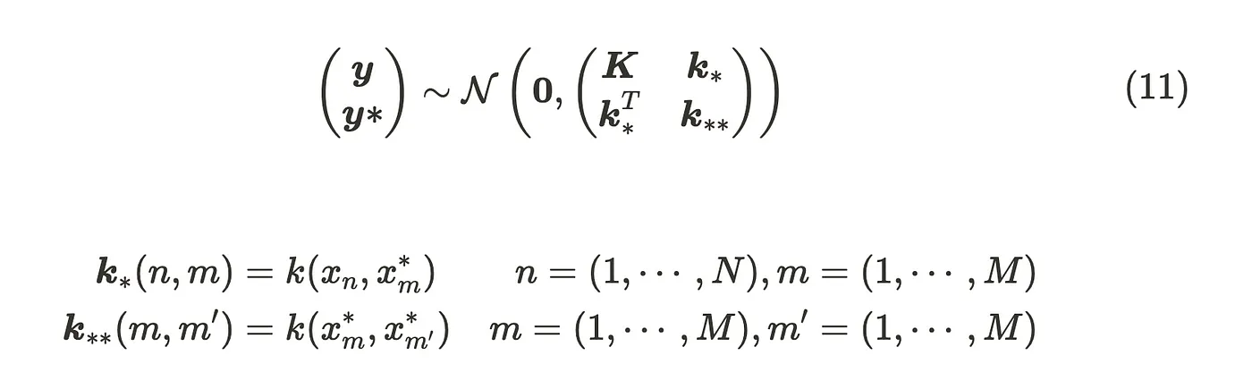
Please remember the formula (2), the parameters of the conditional multivariate Gaussian distribution.

When we apply this formula to the formula (11), the parameters will be as follows:

This is the updating formula for the Gaussian process regression model. When we want to sample from it, we use the lower triangular matrix derived from the Cholesky decomposition.

You can check the detailed theoretical explanation from [4]. However, in the practical situation, you don’t need to implement the Gaussian process regression from scratch because there are already good libraries in Python.
In the following small sections, we will learn how to implement the Gaussian process using the Gpy library. You can easily install it via pip.
Example : Gaussian process model for one dimensional data
We will use a toy example data generated from the sin function with Gaussian noise.
# Generate the randomized sample

X = np.linspace(start=0, stop=10, num=100).reshape(-1, 1)
y = np.squeeze(X * np.sin(X)) + np.random.randn(X.shape[0])
y = y.reshape(-1, 1)
We use the RBF kernel because it is very flexible and easy to use. Thanks to the GPy, we can declare the RBF kernel and Gaussian process regression model with only a few lines.
# RBF kernel
kernel = GPy.kern.RBF(input_dim=1, variance=1., lengthscale=1.)

# Gaussian process regression using RBF kernel
m = GPy.models.GPRegression(X, y, kernel)
The x point refers to the input data, the blue curve does the expected values of the Gaussian process regression model at that point, and the light blue shaded region does the 95% confidence interval.
As you can see, the area with many data points has a shallower confidence interval, but the area with a few points has a broader interval. Thus, if you were an engineer in the manufacturing industry, you could know where you don’t have enough data, but the data region (or experimental condition) is plausible to have target values.
Example : Gaussian process model for multiple dimensional data
We will use the diabetes dataset from the scikit-learn sample dataset.
# Load the diabetes dataset and create a dataframe
diabetes = datasets.load_diabetes()
df = pd.DataFrame(diabetes.data, columns=diabetes.feature_names)
This dataset is already preprocessed (normalized), so we can directly implement the Gaussian process regression model. We can also use the same class for multiple inputs.
# dataset
X = df[['age', 'sex', 'bmi', 'bp']].values
y = df[['target']].values

# set kernel
kernel = GPy.kern.RBF(input_dim=4, variance=1.0, lengthscale=1.0, ARD = True)

# create GPR model
m = GPy.models.GPRegression(X, y, kernel = kernel)
The result is the table below.

As you can see, there is much room for improvement. The easiest step to improve the prediction result is to gather more data. If it is impossible, you can change the choice of kernels or the hyperparameter optimization. I will later paste the code I used, so feel free to change and play it!
You can reproduce the visualization and GPy experiments using the code below.
We have discussed the mathematical theorem and the practical implementation of the Gaussian process. This technique is beneficial when you have a small amount of data. However, since the computation amount depends on the number of data, please remember that it is not suitable for large data. Thank you for reading!
References
[1] Mochihashi, D., Oba, S., ガウス過程と機械学習, 講談社
[2]https://www.khoury.northeastern.edu/home/vip/teach/MLcourse/3_generative_models/lecture_notes/Marginal and conditional distributions of multivariate normal distribution.pdf
[3] Hui, J., Kernels for Machine Learning, Medium