Faster R-CNN: Object Detection
This is the 2nd Installment of our Object Detection Series which Ayush Raj started with the introductory blog on his channel. Check out that Blog here: Series Introductory Blog.
Introduction
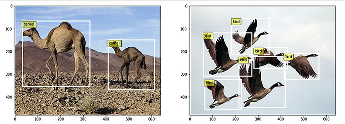
Object detection consists of two separate tasks: classification and localization. R-CNN stands for Region-based Convolutional Neural Network. The key concept behind the R-CNN series is region proposals. Region proposals are used to localize objects within an image. The R-CNN which was initially designed, has evolved over the years to Fast R-CNN and then on to the Faster R-CNN architecture. The goal of this article is to cover the workings of the Faster R-CNN architecture.
Problems with Fast R-CNN
Although Fast R-CNN overcame some of the problems of the R-CNN, the region of proposals was still calculated via the Selective Search algorithm and the inference time was still quite slow. So to overcome these issues, Faster R-CNN came up with the concept of Region Proposal Networks (RPNs).
Faster R-CNN
Faster R-CNN is an Object Detection architecture presented by Ross Girshick, Shaoqing Ren, Kaiming He, and Jian Sun in 2015, and is one of the famous Object Detection architectures that uses Convolution Neural Networks(CNNs).
Components of Faster R-CNN:
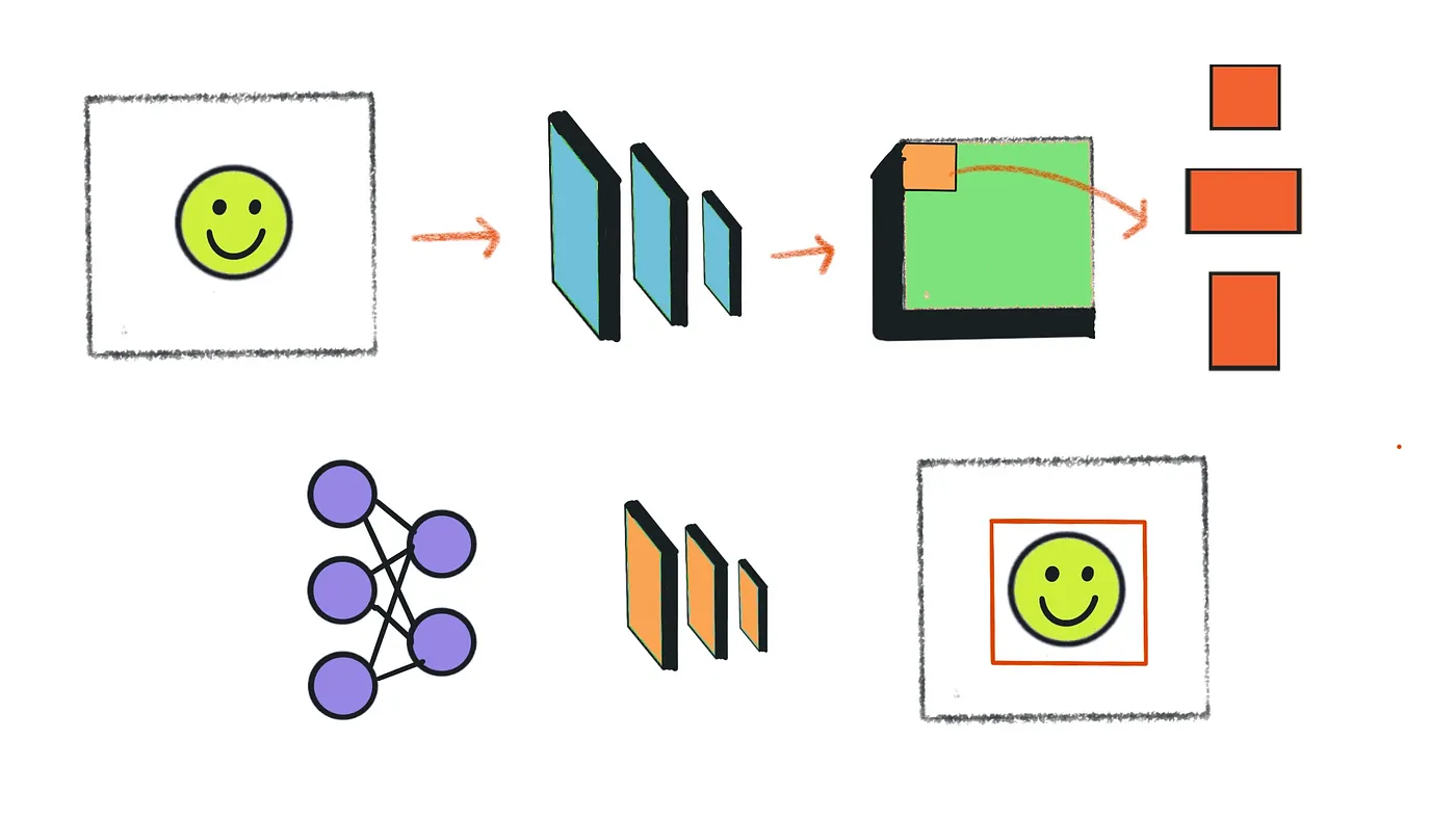
The main components of Faster R-CNN are the Region Proposal Network and the ROI pooling coupled with a Classifier and Regressor Head to obtain the predicted class labels and bounding box locations.
Faster R-CNN is composed of 3 parts:
The Convolution Layers:
In these layers we train filters to extract the appropriate features in the image, for example, let’s say that we are going to train these filters to extract the appropriate features for a human face, then these filters are going to learn through training shapes and colors that only exist in the human face.
Convolution networks are generally composed of Convolution layers, pooling layers, and a last component which is the fully connected layer or another extended thing that will be used for an appropriate task like classification or detection.
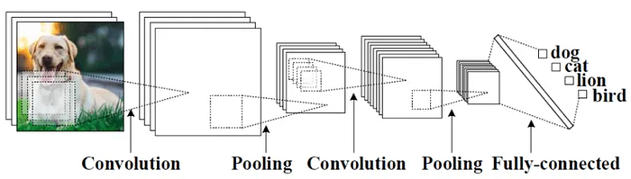
As you know, we compute convolution by sliding an N*N Filter all along our three-dimensional input image and the result we obtain is a two-dimensional matrix called a feature map. Let’s understand it using an illustration:
Let's consider a filter of size 3x3 and an image of size 5x5. We perform an element-wise multiplication between the image pixel values that match the size of the kernel and the kernel itself and sum them up. This provides us with a single value for the feature map.
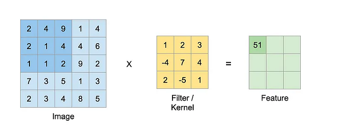
2*1 + 4*2 + 9*3 + 2*(-4) + 1*7 + 4*4 + 1*2 + 1*(-5) + 2*1 = 51
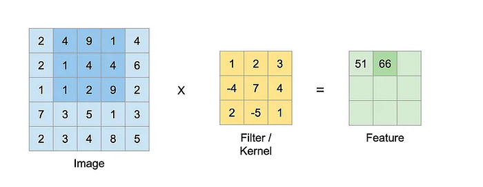
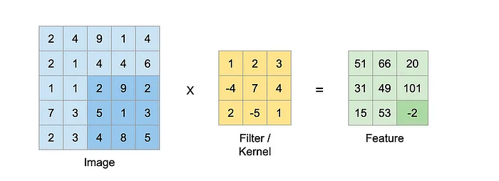
Filter continues to run further on the image and produces new values as shown below.
Once an image passes through the backbone network, it gets down-sampled along the spatial dimension. The output is a feature-rich representation of the image.

The images that we’ve taken here for illustration, if we pass these Images of size (640, 480) through the backbone network, we get an output feature map of size (15, 20). So the image has been down-scaled by (32, 32).
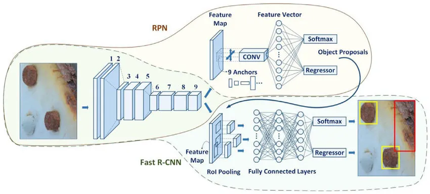
Region Proposal Network (RPN):
RPN is a small neural network sliding on the last feature map of the convolution layers and predicting whether there is an object or not and also predicting the bounding box of those objects.
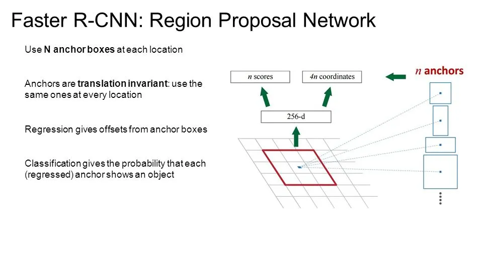
The RPN is responsible for returning a good set of proposals from the generated image anchors in the previous step. The RPN consumes the feature map generated by the image feature extractor and passes it through two parallel convolution layers to give two sets of outputs.
The first convolution layer gives the bounding box regressor outputs. The purpose of these outputs is not to pinpoint the direct locations of the bounding boxes themselves, but rather to predict the offset and scales, which are to be applied over the image anchors to refine the predictions.
The second layer also outputs a classification output indicating the probability of the bounding boxes to be foreground or background.
Anchors
Anchors are potential bounding box candidates where an object can be detected. They are a predefined set of boxes before the start of training, based on a combination of aspect ratios and scales, and placed throughout the image. Faster R-CNN utilizes 3 aspect ratios and 3 scales generating 3*3 = 9 combinations of Anchor Boxes.
Let's consider an aspect ratio of 0.5 and scale combinations of [8,16, 32]. The final down-sampled image stride size, after passing the image through a conv-pool VGG network is 16. Now the resulting combinations with the above would be:

Here we get 3 rectangles with a width larger than its height. Similarly, by considering a ratio of 1, we get 3 variations of a square, and with a ratio of 2, there would be 3 variations of a rectangle with a height larger than the width. This forms the base anchor with a total of 9 variations.
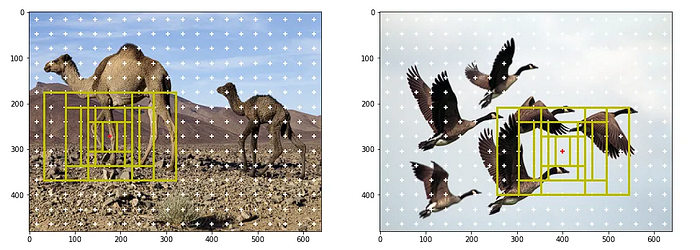
Now that we have obtained the base anchor, the next step would be to generate all the possible anchors for the image.
Each anchor is denoted by (x1, y1, x0, y0) where x1, y1 are the top left corners and x0, y0 are the bottom right corners of a box.
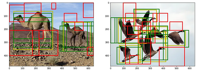
Positive and Negative Anchor Boxes
Positive anchor boxes contain an object and negative anchor boxes do not. To sample positive anchor boxes, we select the anchor boxes that have an IoU of more than 0.7 with any of the ground truth boxes or those that have the highest IoU for every ground truth box. When anchor boxes are poorly generated, condition 1 fails, so condition 2 comes to the rescue as it selects one positive box for every ground truth box. To sample negative anchor boxes, we select the anchor boxes that have an IoU less than 0.3 with any of the ground truth boxes. Usually, the number of negative samples will be far higher than the number of positive samples.

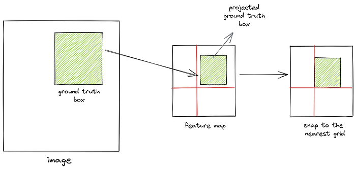
IoU is computed in the feature space between the generated anchor boxes and the projected ground truth boxes. To project a ground truth box onto the feature space we simply divide its coordinates by the scale factor. Now, when we divide the coordinates by the scale factor, we round off the value to the nearest integer. This essentially means we’re “snapping” the ground truth box to the nearest grid in the feature space. So if the difference in scale of image space and feature space is high, we would not get accurate projections. Hence, it’s important to work with high-resolution images in object detection.
Computing Offsets
The positive anchor boxes do not exactly align with the ground truth boxes. So we compute offsets between the positive anchor boxes and the ground truth boxes and train a neural network to learn these offsets. We’re teaching the network to learn how much the anchor box is off from the ground truth box. We’re not forcing it to predict the exact location and scale of the anchor box. To do so, we need to map every positive sample to its corresponding ground truth box. It’s important to note that a positive anchor box maps to only one ground truth box, while multiple positive anchor boxes can map to the same ground truth box. Then for each anchor box, we select the ground truth box it overlaps with the most.
Finally, we select negative samples by sampling the anchor boxes which have an IoU less than the given threshold with all of the ground truth boxes. Since negative samples far outweigh positive samples in number, we randomly select a few of them to match the count.
The Proposal Module:
Every point in the feature map is considered an anchor, and every anchor generates boxes of different sizes and shapes. We want to classify each of these boxes as object or background. Moreover, we want to predict their offsets from the corresponding ground truth boxes.
How can we do that?
The solution is to use 1x1 convolution layers. Now, a 1x1 a convolutional layer does not increase the receptive field. Their function is not to learn image-level features. They are rather used to change the number of filters or to serve as a regression or classification head.
So we take two 1x1 convolutional layers and use one of them to classify each anchor box as object or background. Let’s call this the confidence head. So, given a feature map, we convolve a kernel of size 1x1 to get an output. Essentially, each output filter represents the classification score of an anchor box.

In a similar way, the other 1x1 convolutional layer takes the feature map and produces an output where the output filters represent the predicted offsets of the anchor boxes. This is called the regression head.
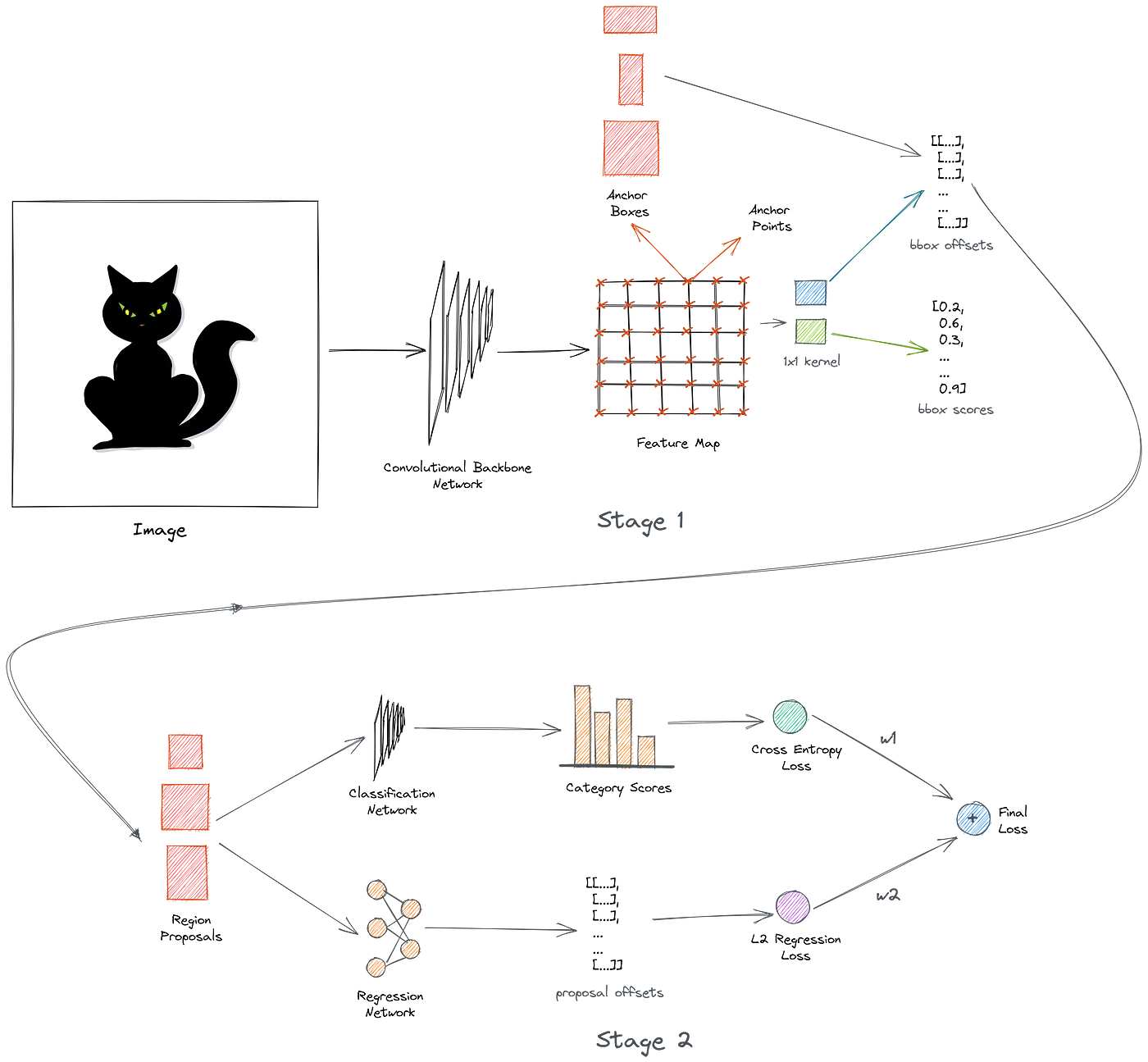
Concluding RPN
The region proposal network is stage 1 of the detector which takes the feature map and produces region proposals. Here we combine the backbone network, the sampling module, and the proposal module into the region proposal network.
During both training and inference, the RPN produces scores and offsets for all the anchor boxes. However, during training, we select only the positive and negative anchor boxes to compute classification loss. To compute L2 regression loss, we only consider the offsets of positive samples. The final loss is a weighted combination of both of these losses.
During inference, we select the anchor boxes with scores above a given threshold and generate proposals using the predicted offsets. We use a sigmoid function to convert the raw model logits to probability scores.
The proposals generated in both cases are passed to the second stage of the detector.
The Classification Module:
In the second stage, we receive region proposals and predict the category of the object in the proposals. This can be done by a simple convolutional network, but there’s a catch: all proposals do not have the same size. Now, you may think of resizing the proposals before feeding them into the model like how we usually resize images in image classification tasks for every proposal which are many, but don’t you think this is a naive approach? Don’t you?
Here’s a smarter way to resize: we divide the proposals into roughly equal subregions (they may not be equal) and apply a max pooling operation on each of them to produce outputs of same size. This is called ROI pooling.

Let’s just understand this by example,
And I’ve taken this example specifically to emphasize that regions can be divided into unequal parts!
Let’s consider a small example to see how it works. We’re going to perform region of interest pooling on a single 8×8 feature map, one region of interest, and an output size of 2×2. Our input feature map looks like this:

Let’s say we also have a region proposal (top left, bottom right coordinates): (0, 3), (7, 8). In the picture, it would look like this:

Normally, there’d be multiple feature maps and multiple proposals for each of them, but we’re keeping things simple for the example.
By dividing it into (2×2) sections (because the output size is 2×2) we get:
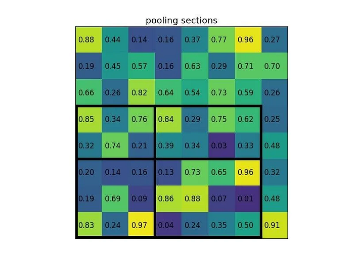
Note that the size of the region of interest doesn’t have to be perfectly divisible by the number of pooling sections (in this case our RoI is 7×5 and we have 2×2 pooling sections).
The max values in each of the sections are:
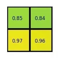
And that’s the output from the Region of Interest pooling layer. Here’s our example presented in the form of a nice animation:
So, I hope that you get the intuition and significance of RoI Pooling now. It takes care of the fixed size input constraint of next CNNs. Hence, gives major convenience to us.
Pooling consists of decreasing the quantity of features in the features map by eliminating pixels with low values.
Once the proposals have been resized using ROI pooling, we pass them through a convolutional neural network consisting of a convolutional layer followed by an average pooling layer followed by a linear layer that produces category scores.
During inference, we predict the object category by applying soft max function over the raw model logits and selecting the category with highest probability score. During training, we compute the classification loss using cross-entropy.
Non-Maximum Suppression
Non-maximum suppression (NMS) is applied over the predicted bounding boxes using their predicted scores as criteria for filtration. In this technique, we first consider the bounding box with the highest classification score. Then we compute IoU of all the other boxes with this box and remove the ones that have a high IoU score. These are the duplicate bounding boxes that overlap with the “original” ones. We repeat this process for the remaining boxes as well until all the duplicates get removed.
The Faster R-CNN Model
We put together the region proposal network and the classification module to build the final end-to-end Faster R-CNN Model.
Losses
There are four sets of losses in total for the model to train. These 4 losses are obtained from 2 layers: RPN and RoI Pool/Head layer.
RPN
The IoU between the ground truth bounding box and the image anchors is calculated.
- Bounding Boxes Offsets/Scales:-
The predicted offsets/scales are decoded with the image anchors to get the final bounding boxes. Similarly, the image anchors are encoded with their maximum IOU ground truth bounding box to obtain the offsets/scale differences. - Bounding Boxes Confidence Scores:-
The predicted confidence scores indicate the presence of an object and whether it is background or foreground. For the ground truth labels, those with IOUs, above a positive threshold are marked with label 1 and below a negative threshold with label 0. The remaining are marked as -1 indicating that they can be ignored.
RoI
The IoU between the ground truth bounding box (GTBb) and the selected RoI(s) are calculated.
- Bounding Box Refinement:
The VGG head predicts “offsets/scales” for the selected ROIs. These are used to refine the initial RoI positions and sizes based on the predicted adjustments.
To calculate the ground truth offsets/scales, the selected RoI is encoded with its corresponding maximum IoU Ground Truth Bounding Boxes (GTBb). This means finding the GTBb with the highest IoU among all GTBbs for that particular RoI. The predicted offsets/scales are applied to the selected RoIs, potentially improving their accuracy.
2. Bounding Boxes Labels:
The VGG head predicts class labels for the selected RoIs. Each RoI requires a ground truth class label for calculating the loss function. Similar to bounding box refinement, the RoI is again associated with its maximum IoU GTBb.
The ground truth label of this assigned GTBb is then used as the label for the RoI. By associating each RoI with its most relevant GTBb, the model ensures its learning to classify objects based on their true presence in the image.
Faster R-CNN uses Smooth L1-Loss (that we generally know as Mean Absolute Error(MAE) Loss) for the regressors and Cross-Entropy for the classifier to calculate the loss. The loss from these four layers are accumulated and backpropagated to train the overall model.
Conclusion:
The article provides a comprehensive overview of Faster R-CNN, a groundbreaking object detection architecture, still used for its most better accuracy results. It begins by introducing the concept of object detection and the evolution of R-CNN models, leading to the development of Faster R-CNN. The article delves into the key components of Faster R-CNN, including the Region Proposal Network (RPN), Anchor Boxes, proposal module, and classification module. It explains the intricate workings of each component, such as how RPN generates region proposals and how the classification module predicts object categories. Additionally, the article covers important concepts like Non-Maximum Suppression in a briefer sense, RoI Pooling, and loss functions used in training the model. Overall, it offers a thorough understanding of Faster R-CNN’s architecture and its role in advancing object detection capabilities and pipelines in computer vision applications.
Do Follow for more such content!!!