Data Science, Statistics
Descriptive Statistics with Pandas
Statistical concepts with examples, formula, and python code

Contents
- Estimate of Location
- Mean
- Trimmed Mean
- Weighted Mean
- Median
- Mode
2. Estimate of Variability
- Deviation
- Mean Absolute Deviation
- Median Absolute Deviation
- Variance
- Standard Deviation
- Interquartile Range
3. Correlation
Understanding the dataset
We will be using simple product details dataset which contains Product ID, Cost Price, and Selling Price to demonstrate various statistical methods.

Imports and Reading data
Most of the statistical methods can be done with Pandas except trimmed mean(scipy) and weighted mean(numpy). Reading product data into a data frame called ‘products’. Seaborn is a graphical plotting library.
import numpy as np
import pandas as pd
from scipy import stats
import seaborn as snsproducts = pd.read_csv('products.csv')
Estimate of Location
When there are several distinct values it is often very helpful to see an estimate of where the data is located or centered. It is also referred to as Measure of Central Tendency. Let’s see different ways of measurement.
- Mean
The most basic estimate of location is the mean of data, simply an average of the values. That is the sum of all the values divided by the total number of values.
Example
Values: 10, 11 , 1, 20, 13
Mean = (10+11+1+20+13)/5 = 11
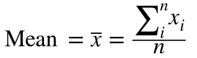
The mean is symbolized as ‘x-bar’, n is the total number of values.
products['Cost Price'].mean()Output: 94.2
2. Trimmed Mean
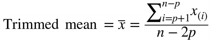
Another variant of mean is trimmed mean. The trimmed mean is nothing but excluding a certain percentage of value from the extreme ends of sorted data whose average needs to be measured.
For example, in a diving tournament, the top score and bottom score from five judges are dropped and the final score is the mean of the remaining three judges. This makes it difficult for a single judge to manipulate the score.
Example
Values: 10, 11 , 1, 20, 13
Sort: 1, 10, 11, 13, 20
After Trimming: 10, 11, 13
Mean = (10+11+13)/= 11.33
Note: Since the values are small in the example there is not much difference between the mean and trimmed mean. When we deal with real-world data trimmed mean makes a difference.
#using stats from scipy
#trimming 10%(0.1) of values from both end od sorted data
#trim_mean() sorts the values internally
stats.trim_mean(products[’Cost Price’], 0.1)Output: 93.625
3. Weighted mean
The weighted mean is another type of mean in which we multiply the value with user-specified weight and dividing their sum with the total weight given.
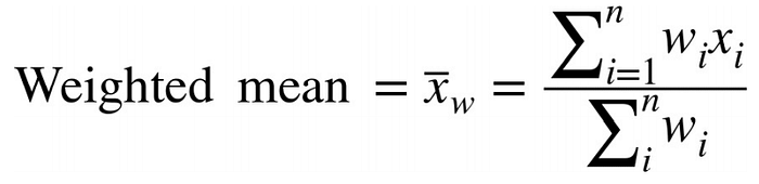
where w is the weight corresponding to the value x.
#generating random weights
weights = [i for i in range(10,20)]#calculating weighted average
np.average(products['Cost Price'], weights=weights)Output: 99.6896551724138
When to use a weighted mean?
- Suppose we are taking an average of multiple sensor readings and two of the sensors are less accurate then it might be feasible to assign less weight to that sensor instead of discarding the reading.
- Suppose we might not have data that represents all the groups in our dataset. To correct that, we can assign a higher weight to the group of values that were underpredicted.
4. Median
Median is nothing but the middle value of the sorted data. If there are an even number of values then the median would be the mean of two values that would divide the sorted data into the equal lower and upper half.
Example 1
Values: 10, 11 , 1, 20, 13
Sort: 1, 10, 11, 13, 20
Median: 11
Example 2
Values: 10, 11 , 1, 20, 13, 5
Sort: 1, 5, 10, 11, 13, 20
Median: (10+11)/2=10.5
products['Cost Price'].median()Output: 93.5
Why median over mean?
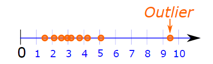
Mean is very sensitive to outliers which may manipulate the estimate of location. For example, we are interested in calculating the average revenue of startup’s that started just before the COVID19 outbreak, we can see that there is one startup company whose revenue is very high as compared to remaining because that startup company was into modern fabrics and soon as the demand for the masks was hyped they started producing masks and hence high revenue. This is considered as an outlier which will result in an inaccurate data summary. During such situations, the median is preferred.
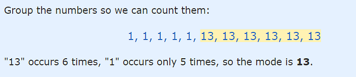
5. Mode
The mode is the simplest of all, the value whose occurrence is highest in the data is the mode. Although the example below has numbers, the mode is summary stats for categorical data, generally not used for numerical.
#value_counts() given number of occurances
#of each unique values in Cost Price column
products['Cost Price'].value_counts()
Estimate of Variability
At the heart of the statistics lies variability. Variability is another dimension in summarizing a feature. Also known as dispersion, measures whether a value is tightly clustered or spread out. Statisticians have defined many ways to measure the dispersion, let’s see each of them.
- Deviation
The deviation is the most widely used estimate of variation. It measures how much a given data point deviates from an estimate of location.
Example
Values: 10, 11 , 1, 20, 13
Mean(estimate of location): 11
Deviation of each value from mean
=10–11, 11–11, 1–11, 20–11, 13–11
= -1, 0, -10, 9, 2
In the above example, it shows how much each value is dispersed from the estimate of location.
2. Mean absolute deviation
Just the deviation values do not make much sense, we need to summarize it to draw some inference and that would be done by calculating the average of these deviations.
Example
Deviation values: -1, 0, -10, 9, 2
Avegare: (-1 + 0 + -10 + 9 + 2)/5 = 0
Surprised? don’t be. The mean of deviations is always zero, the negative values offsets the positive values. To overcome this we take absolute values of deviation.
Absolute deviation values: 1, 0, 10, 9, 2
Average: (1+0+10+9+2)/5=4.4
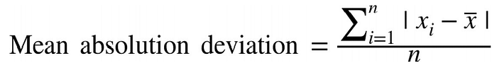
x-bar is the mean, x is individual value, n in the total number of values
#np is alias for numpy
mean = np.mean(products['Cost Price'])
np.mean(np.absolute(products['Cost Price'] - mean))Output: 35.0
3. Median Absolute Deviation
You guessed it right. Use the median in place of the mean to get Median Absolute Deviation. The reason to use is the same, the median absolute deviation is insensitive to outliers.
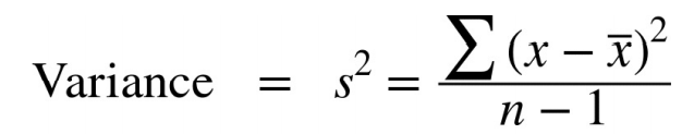
4. Variance
Variance is the average of squared deviation. It is preferred over mean absolute deviation by many statisticians because it is more accurate.
Example
Squared deviation of each value from mean
=(10–11)², (11–11)², (1–11)², (20–11)², (13–11)²
= 1, 0, 100, 81, 4
Variance = (1+0+100+81+4)/(5–1)
=37.2
5. Standard Deviation
We found the variance in the above example is 37.2 but how good or bad is 37.2? what does a variance of 37.2 actually mean? To extract information from variance we calculate the standard deviation. The square root of the variance is the standard deviation. Standard Deviation is the most preferred method to find how the spread the data because the resulting value is on the same scale as the original data.
Example
Variance =37.2
Standard deviation = 6.09
This value looks good. It makes more sense. Now we can tell which value is within one standard deviation (6.09) of the mean.

products['Cost Price'].std()Output: 39.33276835752432
6. Interquartile Range
Another different approach to estimate dispersion is looking at the spread of sorted data. This can be done by calculating the Interquartile Range(IQR) which is the difference between the 25th percentile and 75th percentile.
What is percentile?
Suppose you rank 4th in a class of 20 people by marks obtained which means 80% of the people scored lesser than you. In other words, you are the 80th percentile of the class group.
The other way around, to find the 80th percentile, sort the data and starting from the smallest value proceed 80% of the way towards the largest value to get the 80th percentile.
Example
Values: 3, 1, 5, 3, 6, 7, 2, 9
Sort: 1 ,2, 3, 3, 5, 6, 7, 9
25th percentile: 2.5
75th percentile: 6.5
Interquartile Range: 6.5–2.5 = 4
percentile_75th = products['Cost Price'].quantile(0.75)
percentile_25th = products['Cost Price'].quantile(0.25)
IQR = percentile_75th - percentile_25thOutput: 68.0
Correlation
Correlation is a measure of the joint variability of two variables. The measurement is generally among predictors or between the predictor variable and target variables. Correlation values always range between -1 and 1.
- Variables X and Y are said to be positively correlated(value 1) if Y value increases as X value increases or Y value decreases as X value decreases.
- A correlation value of 0 means that the two variables are independent.
- If Y value decreases as X value increases or vice-versa then the two variables X and Y are said to be negatively correlated.
Let’s see how Cost Price and Selling Price are correlated in our Products dataset. Again, Pandas has a very simple function corr() that picks up numerical columns in the dataset and gives a tabular form of correlation.
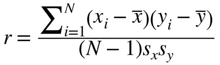
x is an individual value of the variable X, y is an individual value of the variable Y, x-bar is the mean of the variable X, y-bar is the mean of the variable Y, N stands for the total number of values, S(x) is the standard deviation of X and S(y) is the standard deviation of Y.
Note:
Correlation between the same variables is always 1.
products.corr()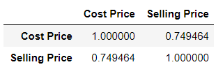
It says that the cost price and selling price are correlated with the value of 0.75. Anything greater than 0.5 can be considered as a positive correlation. Meaning, there high chance that if the cost price of any product increases the selling price also increases or vice-versa. The tabular form is good when we have a lesser column, when we have many columns the tabular form is difficult to read. Seaborn is a visualizing library that can plot the correlation for quick understanding.
#sns is alias to seaborn
#heatmap to plot correlation
sns.heatmap(products.corr(),annot=True)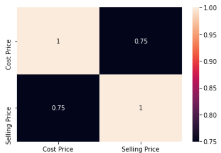
Now, this is easier to interpret.