Creating 3D Videos from RGB Videos

Instructions for generating consistent depthmap and point cloud videos from any RGB videos

Image by the author (edited version of the video frame from stock footage provided by Videvo, downloaded from www.videvo.net)

I’ve always had discontentment with the fact that we archive our digital memories in 2D formats — photographs and videos that, despite their clarity, lack the depth and immersion of the experiences they capture. It’s a limitation that seems arbitrary in an era where machine learning models can be powerful enough to understand the 3Dness of photos and videos.

3D data from images or videos not only lets us experience our memories more vividly and interactively but also offers new possibilities for editing and post-processing. Imagine being able to effortlessly remove objects from a scene, switch out backgrounds, or even shift the perspective to see a moment from a new viewpoint. Depth-aware processing also gives machine learning algorithms a richer context to understand and manipulate visual data.

While searching for methods to generate consistent depth of videos, I found a research paper that suggested a nice approach. This approach involves training two neural networks together using the entire input video: a convolutional neural network (CNN) to predict depth, and an MLP to predict the motion in the scene, or “scene flow”. This flow prediction network is used in a special way where it’s applied repeatedly over different periods of time. This allows it to figure out both small and large changes in the scene. The small changes help to ensure that the motion from one moment to the next is smooth in 3D, while the larger changes help to make sure that the entire video is consistent when seen from different perspectives. This way, we can create 3D videos that are both locally and globally accurate.

The code repo of the paper is publicly available, however, the pipeline for processing arbitrary videos is not entirely explained, and at least for me, it was unclear how to process any video with the proposed pipeline. In this blog post, I will try to fill that gap and give a step-by-step tour of how to use the pipeline on your videos.

You can check my version of the code on my GitHub page, which I will be referring to.

Step 1: Extract frames from the video

The first thing we do in the pipeline is to extract frames from the chosen video. I’ve added a script for this purpose, which you can find at scripts/preprocess/custom/extract_frames_from_video.py. To run the code, simply use the following command in your terminal:

python extract_frames_from_video.py ^
  -- video_path = 'ENTER YOUR VIDEO PATH HERE' ^
  -- output_dir = '../../../datafiles/custom/JPEGImages/640p/custom/' ^
  -- resize_factor = 0.5

Using the resize_factor argument, you can downsample or upsample your frames.

I have selected this video for my tests. Initially, it had a resolution of 1280x720, but to speed up processing in subsequent steps, I downsized it to 640x360 using a resize_factor of 0.5.

Step 2: Segment a foreground object in the video

The next step in our process requires segmenting or isolating one of the main foreground objects in the video, which is crucial for estimating the camera’s position and angle within the video. The reason? Objects closer to the camera significantly influence pose estimation more than those farther away. To illustrate, imagine an object one meter away moving 10 centimeters — this would translate to a sizeable change in the image, perhaps dozens of pixels. But, if the same object were 10 meters away and moved the same distance, the image change would be far less noticeable. Consequently, we’re generating a ‘mask’ video to focus on the relevant areas for pose estimation, simplifying our calculations.

I preferred Mask-RCNN for segmenting the frames. You can use other segmentation models of your preference as well. For my video, I decided to segment the person on the right as he stays in the frame during the entire video and seems close enough to the camera.

To generate the mask video, some manual adjustments specific to your video are necessary. Since my video contains two individuals, I began by segmenting the masks for both persons. Afterward, I extracted the mask for the person on the right through hardcoding. Your approach may vary depending on the foreground object you’ve selected and its position within the video. The script responsible for creating the mask can be found at ./render_mask_video.py. The section of the script where I specify the mask selection process is as follows:

    file_names = next(os.walk(IMAGE_DIR))[2]
    for index in tqdm(range(0, len(file_names))):
        image = skimage.io.imread(os.path.join(IMAGE_DIR, file_names[index]))
        # Run detection
        results = model.detect([image], verbose=0)
        r = results[0]
        # In the next for loop, I check if extracted frame is larger than 16000 pixels, 
        # and if it is located minimum at 250th pixel in horizontal axis.
        # If not, I checked the next mask with "person" mask.
        current_mask_selection = 0
        while(True):
            if current_mask_selection<10:
                if (np.where(r["masks"][:,:,current_mask_selection]*1 == 1)[1].min()<250 or 
                    np.sum(r["masks"][:,:,current_mask_selection]*1)<16000):
                    current_mask_selection = current_mask_selection+1
                    continue
                elif (np.sum(r["masks"][:,:,current_mask_selection]*1)>16000 and 
                      np.where(r["masks"][:,:,current_mask_selection]*1 == 1)[1].min()>250):
                    break
            else:
                break
        mask = 255*(r["masks"][:,:,current_mask_selection]*1)
        mask_img = Image.fromarray(mask)
        mask_img = mask_img.convert('RGB')
        mask_img.save(os.path.join(SAVE_DIR, f"frame{index:03}.png"))

The original video and the mask video are visualized side-by-side in the following animation:

(Left) Stock footage provided by Videvo, downloaded from www.videvo.net | (Right) Masked video created by the author

Step 3: Estimate camera pose and intrinsic parameters

After creating the mask frames, we now proceed with the computation of camera pose and intrinsic estimation. For this, we use a tool called Colmap. It is a multi-view stereovision tool that creates meshes from multiple images and also estimates camera movements and intrinsic. It has a GUI as well as a command line interface. You can download the tool from this link.

Once you start the tool, you will press “Reconstruction” on the top bar (see figure below), then “Automatic reconstruction”. In the pop-up window,

• enter ./datafiles/custom/triangulation to “Workspace folder”
• enter ./datafiles/custom/JPEGImages/640p/custom to “Image folder”
• enter ./datafiles/custom/JPEGImages/640p/custom to “Image folder”
• enter ./datafiles/custom/Annotations/640p/custom to “Mask folder”
• tick “Shared intrinsics” option
• click “Run”.

The computation can take a while depending on how many images you have and the resolution of the images. Once the computation is over, click “Export model as text” under “File” and save the output files in ./datafiles/custom/triangulation. It will create two text and one mesh (.ply) file.

Instructions for Colmap — Image by the author

This step is not over yet, we have to process the outputs of Colmap. I’ve written a script to automate it. Simply, run the following command in the terminal:

python scripts/preprocess/custom/process_colmap_output.py

It will create “custom.intrinsics.txt”, “custom.matrices.txt” and “custom.obj”.

Output files of Colmap — Image by the author

Now we are ready to proceed with the dataset generation for the training.

Step 4: Prepare the dataset for training

The training requires a dataset that consists of depth estimations of each frame by MiDas, corresponding cross-frame flow estimations, and depth sequences. The scripts for creating these were provided in the original repo, I only changed the input and output directories in them. By running the command below, all the required files will be created and placed in the appropriate directories:

python scripts/preprocess/custom/generate_frame_midas.py  &
python scripts/preprocess/custom/generate_flows.py  &
python scripts/preprocess/custom/generate_sequence_midas.py  

Before training, please check if you have .npz and .pt files in datafiles/custom_processed/frames_midas/custom , datafiles/custom_processed/flow_pairs/custom and datafiles/custom_processed/sequences_select_pairs_midas/custom. After the verification, we can proceed with the training.

Step 5: Training

The training part is straightforward. To train the neural network with your custom dataset, simply run the following command in the terminal:

python train.py --net scene_flow_motion_field ^
 --dataset custom_sequence --track_id custom ^
 --log_time  --epoch_batches 2000 --epoch 10 ^
 --lr 1e-6 --html_logger --vali_batches 150  ^
 --batch_size 1 --optim adam --vis_batches_vali 1 ^
 --vis_every_vali 1 --vis_every_train 1 ^
 --vis_batches_train 1 --vis_at_start --gpu 0 ^
 --save_net 1 --workers 1 --one_way ^
 --loss_type l1 --l1_mul 0 --acc_mul 1 ^
 --disp_mul 1 --warm_sf 5 --scene_lr_mul 1000 ^
 --repeat 1 --flow_mul 1 --sf_mag_div 100 ^
 --time_dependent --gaps 1,2,4,6,8 --midas ^
 --use_disp --logdir 'logdir/' ^
 --suffix 'track_{track_id}' ^
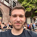
 --force_overwrite

After training the neural network for 10 epochs, I observed that the loss began to saturate, and as a result, I decided not to continue training for additional epochs. Below is the loss curve graph of my training:

Loss vs. epoch curve — Image by the author

Throughout the training, all checkpoints are stored in the directory ./logdir/nets/. Furthermore, after every epoch, the training script generates test visualizations in the directory ./logdir/visualize. These visualizations can be particularly helpful in identifying any potential issues that might have occurred during training, in addition to monitoring the loss.

Step 6: Create depthmaps of each frame using the trained model

Using the latest checkpoint, we now generate the depth map of each frame with test.py script. Simply run the following command in the terminal:

python test.py --net scene_flow_motion_field ^
 --dataset custom_sequence --workers 1 ^
 --output_dir .\test_results\custom_sequence ^
 --epoch 10 --html_logger --batch_size 1 ^
 --gpu 0 --track_id custom --suffix custom ^
 --checkpoint_path .\logdir

This will generate one .npz file for each frame(a dictionary file consisting of RGB frame, depth, camera pose, flow to next image, and so on), and three depth renders (ground truth, MiDaS, and trained network’s estimation) for each frame.

Step 7: Create point cloud videos

In the last step, we load the batched .npz files frame-by-frame and create colored point clouds by using the depth and RGB information. I use the open3d library to create and render point clouds in Python. It is a powerful tool with which you can create virtual cameras in 3D space and take captures of your point clouds with them. You can also edit/manipulate your point clouds; I applied open3d’s built-in outlier removal functions to remove flickery and noisy points.

While I won’t delve into the specific details of my open3d usage to keep this blog post succinct, I have included the script, render_pointcloud_video.pywhich should be self-explanatory. If you have any questions or require further clarification, please don’t hesitate to ask.

Here is what the point cloud and depth map videos look like for the video I processed.

(Left) Stock footage provided by Videvo, downloaded from www.videvo.net | (Right) Depthmap video created by the author | (Bottom) Colorized point cloud video created by the author

A higher-resolution version of this animation is uploaded to YouTube.

Well, depth maps and point clouds are cool, but you might be wondering what you can do with them. Depth-aware effects can be remarkably potent when compared to traditional methods of adding effects. For instance, depth-aware processing enables the creation of various cinematic effects that would otherwise be challenging to achieve. With the estimated depth of a video, you can seamlessly incorporate synthetic camera focus and defocus, resulting in a realistic and consistent bokeh effect.

Moreover, depth-aware techniques offer the possibility of implementing dynamic effects like the “dolly zoom”. By manipulating the position and intrinsics of the virtual camera, this effect can be applied to generate stunning visual sequences. Additionally, depth-aware object insertion ensures that virtual objects are realistically fixed within videos, maintaining consistent positions throughout the scenes.

The combination of depth maps and point clouds unleashes a world of possibilities for captivating storytelling and imaginative visual effects, propelling the creative potential of filmmakers and artists to new heights.

Right after clicking the “publish” button of this article, I will roll up my sleeves and work on making such effects.

Have a great day ahead!