Data Structures and Algorithms Revisited: Part 1

Hello, I’m Kosuke Kuzuoka, an AI research engineer at DeNA Co., Ltd. I recently had a chance to revisit data structures and algorithms, and thought that this would be a good time to share my knowledge and the implementation written in python.
I am writing a series of blog posts, covering topics from the basics of data structures and algorithms to advanced computer science. This blog post is meant for beginners or people who want to learn the basics about CS topics. All the code used in this series is in this Github repository. Let’s dive in!
UPDATED: It’s has been a while since I started this blog post series. I have been working on this series hard, and publishing a new post every week! Here are all the links to the posts published in this series so far. Enjoy 😎
What are Data Structures?
In short, data structures are the ways of storing data in your computer. I assume you know about arrays and lists. An array is a data structure that can store a big chunk of data. You can do a lot of things with arrays, but arrays have some cons as well. In some cases, other data structures like a linked list is better, and sometimes not.
One good property of an array is that it has constant time lookup if you know the index. Constant time lookup means that no matter how much data you have in the array, it will take roughly the same amount of time to get data from the array if you know the index. Let’s look at some examples.

I created 1k arrays with sizes ranging from 1 to 1k, then I picked a random index which is in the range and calculated how many times it took to look up an element from the array. You can see that the lookup time doesn’t really change as the number of elements increases in the array. This means that there is almost no correlation between the time it takes for the lookup and the number of elements in the array.
But arrays have some cons as well. Arrays have linear time when you insert an element into it, while the other data structures like linked-lists have constant time. I won’t go into too much detail since both data structures will be explained in a later post in this blog series. The takeaway here is that you can write more efficient code if you have a good understanding of data structures and algorithms.
What are Algorithms?
In short, algorithms are the ways of solving problems using different types of data structures. Algorithms can be very difficult to understand, but let’s look at a simple example to understand what an algorithm looks like. Below is an example question asked on LeetCode.
Given an array of integers, return indices of the two numbers such that they add up to a specific target.You may assume that each input would have exactly one solution, and you may not use the same element twice.Given nums = [2, 7, 11, 15], target = 9,Because nums[0] + nums[1] = 2 + 7 = 9,
return [0, 1].
The problem you need to solve here is pretty obvious. You basically need to find a pair of numbers that add up to the target value and return the indices of both two numbers. A simple algorithm you can come up with is to have one loop that goes through the numbers one by one, and another loop for checking whether the pair of numbers add up to the target or not. Let’s look at the naive approach to solve this problem in code.
This code obviously works, but it has two loops — one for checking each number and the other one for checking if any number in the array add up to the target value. In fact you can remove the inner loop to clean up the code if you know other data structures, such as using hash maps instead of using arrays. Let’s write the algorithm without the inner loop, instead using hash maps.
In fact both of these algorithms solve this particular problem. Both of them produce the same result. The important thing here is that if you have a good understanding of data structures and algorithms, then you can write very efficient code. But how do you really know how much faster your efficient algorithm runs? This is where Big-O notation comes into play!
What is Big-O notation?
I introduced two algorithms to solve a simple problem. Both of them solve the problem but one of them runs much faster than the other, and I want to show you how to prove that this is the case.

I ran both functions from above with exactly the same input and target. The result is that the optimal approach runs slightly faster than the other function, but the difference between them is really insignificant. Now let’s increase the size of an array to see what happens.

You can clearly see the difference between the two functions is more significant than before. Can you guess why? The answer to that question is that the runtime of the naive approach grows exponentially as the size of the array increases. Big-O notation is great for expressing the relationship of runtime and the size of an array.
Big-O notation indicates the efficiency of your algorithm given an input. Let’s imagine the size of an input array is N. How many times do you think the loop runs through for the naive approach? The outer loop runs through 0 to N and the inner loop runs through i + 1 to N. This is very common behavior for algorithms, and the total amount of times the loop runs is N(N-1)/2 times. This is exactly the same as saying “If the size of an input is N, then the run time for the function is going to be N(N-1)/2”, and this is very close to the definition of Big-O notation with one more modification — which you would like for sure ;)
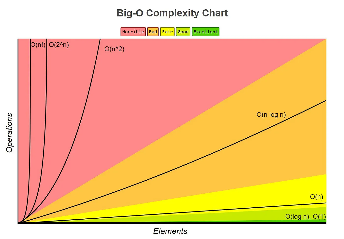
In fact Big-O notation doesn’t care about exact runtime, but the approximate runtime. If you do some math for the runtime that I defined above, it would become N²-N/2. Big-O only cares about the most significant term of the equation and ignores everything else. So the runtime for the naive approach and optimal approach becomes O(N²) and O(N) respectively. There are other metrics you can use to explain the complexity of your algorithms, such as Big-Ω or Big-Θ. But Big-O is the most commonly used one among those, so I won’t explain how Big-Ω or Big-Θ differ from Big-O. The takeaway from this section is that with Big-O notation, you can explain the efficiency for your algorithm.
Conclusion
In this blog post, I shared more information about data structures and algorithms. It’s always better to write efficient programs in terms of runtime and space on your computer. You might not use those algorithms in your work, but sometimes it really helps to write efficient software, so it’s definitely worth the time. You might be learning the data structures and algorithms for your upcoming interview or for your college classes. In either case, I hope this blog post helped you understand the basics of the topic.
In the next blog post of this series, I will talk about some data structures which are widely used for software development. Thanks a lot for reading through this blog post. I will do my best to write the next post ASAP, but in the meantime, make sure you leave 50 claps to motivate my next post ;)
