
Centralized optimization model for multi-microgrids [Part 2]
In the previous blog, we developed an optimization model for a muli-microgrid system. This blog will cover the CPLEX implementation of that problem.
Defining environment and model
To begin, first, we should create a CPLEX environment and a model inside that environment using “IloEnv” and “IloModel”.
    IloEnv env;
    IloModel model(env);
Input Data
Then, we define the input data; The constant parameters such as electricity market price, forecasted wind turbine output, load profile of each microgrid, diesel generator, and battery capacity limits and efficiencies. These are specified using C++ data types (int, float, and double), and the profiles are stored in a 1D or 2D array data structure.
    int T = 24; // Number of time intervals
    int numMgs = 2; // Number of microgrids

    float chargeEff = 0.95; // Charging efficiency
    float dischargeEff = 0.95; // Discharging efficiency
    int chgMax = 50; // Maximum charging rate of battery
    int dchMax = 50; // Maximum discharging rate of battery


    int capDg = 150; // Capacity of diesel generator
    int dgMin = 50; // Minimum power output of diesel generator
    int dgMax = 150; // Maximum power output of diesel generator

    int* capBatt = new int[numMgs] { 100, 100 }; // Capacity of battery in each microgrid

    double* Cbuy = new double[T] { 90, 90, 90, 90, 90, 90, 110, 110, 110, 110, 110, 125, 125, 125, 125, 125, 125, 125, 110, 110, 110, 110, 110, 110 }; // Cost of buying electricity
    double* Csell = new double[T] { 70, 70, 70, 70, 70, 70, 90, 90, 90, 90, 90, 105, 105, 105, 105, 105, 105, 105, 90, 90, 90, 90, 90, 90}; //selling price to grid w.r.t time
    int costdg = 80; // Cost of diesel generator

    double** load = new double* [numMgs]; // Load of each microgrid
    load[0] = new double[T] {169, 175, 179, 171, 181, 190, 270, 264, 273, 281, 300, 320, 280, 260, 250, 200, 180, 190, 240, 280, 325, 350, 300, 250};
    load[1] = new double[T] {130, 125, 120, 120, 125, 135, 150, 160, 175, 190, 195, 200, 195, 195, 180, 170, 185, 190, 195, 200, 195, 190, 180, 175};

    double** Pwt = new double* [numMgs]; // Wind turbine power generation
    Pwt[0] = new double[T] {10, 15, 20, 23, 28, 33, 35, 34, 70, 80, 90, 100, 100, 100, 100, 40, 50, 60, 70, 80, 90, 100, 100, 100};
    Pwt[1] = new double[T] { 70, 80, 90, 100, 100, 35, 34, 70, 80, 90, 100, 100, 100, 100, 40, 50, 60, 70, 80, 90, 100, 100, 100};
Decision Variables
Our decision variables should be in a 2D form as we have to find the optimal value for all microgrids (microgrid as dim-1) over the day horizon (time as dim-2). However, the CPLEX does not provide a direct way of creating 2D variables. To do so, we have to create a new data structure for 2D decision variables:
typedef IloArray<IloNumVarArray> NumVar2D;Now we will use the alias “NumVar2D” for defining our decision variables. The below code snippet shows the definition of 2D decision variables used in our problem, the “for loop” is used to populate these 2D variables with variable arrays of size equal to the dispatching time horizon of the problem.
    NumVar2D Pdg(env, numMgs); // Power output of diesel generator
    NumVar2D Pchg(env, numMgs); // Power charging the battery
    NumVar2D Pdch(env, numMgs); // Power discharging the battery
    NumVar2D Pbuy(env, numMgs); // Power bought from the grid
    NumVar2D Psell(env, numMgs); // Power sold to the grid
    NumVar2D SOC(env, numMgs); // State of charge of the battery

    for (int i = 0; i < numMgs; i++)
    {
        Pdg[i] = IloNumVarArray(env, T, 0, dgMax);
        Pchg[i] = IloNumVarArray(env, T, 0, chgMax);
        Pdch[i] = IloNumVarArray(env, T, 0, dchMax);
        Pbuy[i] = IloNumVarArray(env, T, 0, IloInfinity);
        Psell[i] = IloNumVarArray(env, T, 0, IloInfinity);
        SOC[i] = IloNumVarArray(env, T, 0, 1);
    }
Objective Function
Our objective function is the sum of the cost of the microgrids over the whole dispatching period. We see in the previous blog that the objective function is expressed with double summation (sum over time and microgrids). This can be achieved in CPLEX using nested “for loops” as shown in the below code snippet.
 IloExpr obj(env);
    for (int i = 0; i < numMgs; i++)
    {
        for (int t = 0; t < T; t++)
        {
           obj += costdg * Pdg[i][t] +  Cbuy[t] * Pbuy[i][t] - Csell[t] * Psell[i][t] ;
  }
 }
 model.add(IloMinimize(env, obj));
Constraints
Now we have to implement the constraints of our problem. We will use nested “for loop” and “model.add()” to define the constraint within our model. The first set of constraints in the previous blog Eq. (3) to Eq. (6) can be created as:
 // Limiting Constraints
 for (int i = 0; i < numMgs; i++)
    {
        for (int t = 0; t < T; t++)
        {
         model.add(Pdg[i][t] >= dgMin);
         model.add(Pdg[i][t] <= dgMax);
         model.add(Pchg[i][t] <= chgMax);
         model.add(Pdch[i][t] <= dchMax);
         model.add(Pchg[i][t] >= 0);
         model.add(Pdch[i][t] >= 0);
         model.add(Pbuy[i][t] >= 0);
         model.add(Psell[i][t] >= 0);
         model.add(SOC[i][t] <= 1);
         model.add(SOC[i][t] >= 0);
  }
 }
Next, the power balance constraint (Prev. blog Eq (2) ) is written as given in below code snippet below:
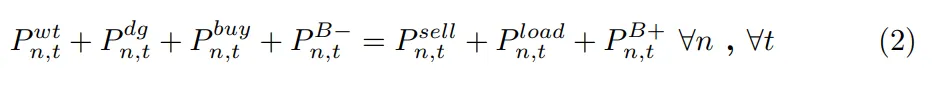
// Power balance
for (int i = 0; i < numMgs; i++)
 {
 for (int t = 0; t < T; t++)
  {
    model.add(Pwt[i][t]+ Pdg[i][t] + Pbuy[i][t] + Pdch[i][t] == Psell[i][t] + load[i][t] + Pchg[i][t]);
  }
 }
The last set of constraints is battery operating constraints (Prev. blog Eq. (7),(8),(9) ). These can be written as:
// Battery  Operating constraints Constraints
for (int i = 0; i < numMgs; i++)
{
  for (int t = 0; t < T; t++)
  {
    if (t == 0)
      {
        model.add(SOC[i][t] == SOC[i][T-1] + (chargeEff * Pchg[i][t] - (1 / dischargeEff) * Pdch[i][t]) / capBatt[i]);
        model.add(Pchg[i][t] <= (1 - SOC[i][T-1]) * capBatt[i] / chargeEff);
        model.add(Pdch[i][t] <= SOC[i][T-1] * capBatt[i] * dischargeEff);
      }
    else
      {
        model.add(SOC[i][t] == SOC[i][t - 1] + (chargeEff * Pchg[i][t] - (1 / dischargeEff) * Pdch[i][t])/ capBatt[i]);
        model.add(Pchg[i][t] <= (1 - SOC[i][t - 1]) * capBatt[i] / chargeEff);
        model.add(Pdch[i][t] <= SOC[i][t - 1] * capBatt[i] * dischargeEff);
      }
   }
}
Note that to handle the Error of “Index out of bounds operation: negative index” for the first time step the “if-else condition” is added.
The SOC at any time is dependent on the previous time SOC and during the start of the day when “t=0”, the previous time “t-1” will throw a negative index error. To deal with this we add the “if-else condition”. So, when the index is zero (start of the day) the SOC value of the last time step (End of the day) would be taken. In theory, we say that the battery SOC level at the start of the day must be equal to the SOC level at the end of the previous day. To express this we add a constraint to our system model:

Finally, to solve our optimization model and obtain the result we create a CPLEX instance using “IloCplex” and pass our model. Then, we call the ‘solve()’ method by invoking ‘cplex.solve()’ to solve the optimization problem. The objective function value can be obtained using “cplex.getObjValue()”.
 IloCplex cplex(model);
 cplex.solve();
 std::cout << "Objective Function Value: " << cplex.getObjValue() << std::endl;
The complete code of this problem is available on my GitHub Repository
In the next blog, we will look into the way to obtain and store the results of each decision variable. Furthermore, we will visualize and analyze those results.
If you have any feedback let me know in the comments below!