SpaceNet 6: Exploring Foundational Mapping at Scale

Preface: SpaceNet LLC is a nonprofit organization dedicated to accelerating open source, artificial intelligence applied research for geospatial applications, specifically foundational mapping (i.e., building footprint & road network detection). SpaceNet is run in collaboration by co-founder and managing partner, CosmiQ Works, co-founder and co-chair, Maxar Technologies, and our partners including Intel AI, Amazon Web Services (AWS), Capella Space, Topcoder, IEEE GRSS, the National Geospatial-Intelligence Agency and Planet.

Introduction

In this third blog (1, 2) of our SpaceNet 6 post-challenge series, we 1)demonstrate that zbigniewwojna’s 1st place algorithm performs well at scale and 2)quantify the value of multiple SAR revisits to the same location. For both of these experiments we are ultimately interested in how well a model performs across a broad area, rather than on a tile by tile basis. Although tile specific metrics are certainly informative of a model’s performance, what we really want to know is “how accurately can this AI algorithm extract buildings across an entire city.” This is important to quantify so we can begin to understand how AI algorithms would perform in a real-world setting where analyzing vast areas is a baseline requirement.

Additionally, the SAR data in the SpaceNet 6 dataset features 204 individual image strips and frequent revisits of the same geographic area. As such, we can also test if model outputs from multiple revisits can be aggregated together to improve the quality of our building footprint predictions. This will inform how many revisits or how much SAR data is required to optimize performance when mapping static objects like buildings. In the figure below we display the distribution of revisits over Rotterdam which ranges from 1 to 30.

The density of aerial SAR collects over Rotterdam in the SpaceNet 6 dataset ranging from 1 to 30. The median number of image strips for the whole area of interest is approximately 15.

In summary, this blog will examine:

1. How well would our 1st place algorithm perform in a real world setting when we want to map buildings across a broad area?
2. How do multiple revisits to the same area affect the quality of building footprint predictions? Is there an optimal number of revisits? How much SAR data is required to optimize performance?

The Workflow

To achieve our analysis goals, we construct the following workflow:

I. Pre-Processing: We rework the SpaceNet 6 training and testing data a bit to ensure that we can achieve the best results at scale. We slightly increase the tile size to 1,200 pixels² and intelligently tile to ensure that each tile has as little blank area as possible. The tiles also include a 20% horizontal overlap which will reduce edge effects and improve stitching quality. We then split the data again to match the same training and testing areas that are present in the SpaceNet 6 dataset.

II. Training and Inference: We train SpaceNet 6 winner zbigniewwojna’s algorithm once more on the larger tiles and then perform inference on our restructured test set (1,200 pixels² tiles).

III. Post-Processing: The final stage of post-processing is aggregating our predicted tiles (model outputs) together to evaluate the effectiveness of the algorithm at city scales. We achieve this by:

1. Merging all tile predictions together that belong to the same SAR image strip.
2. Expand the extent of each SAR image to the full scale of our testing area, padding with 0's.
3. For each of the 204 expanded images, calculate the number of times a pixel is mapped as a building or a non-building.
4. If a pixel is mapped as a building ≥ 50% of the time based upon the number of observations for that pixel, we then classify that pixel as a building. Otherwise, we classify it as a non-building.
5. We then finalize our binarization process and convert the pixel masks back to vectorized geojson format building footprints using the mask_to_poly_geojson function from Solaris.

The Results

Performance differences based upon the scoring format. We compare tiling specific scores vs. the full test area score- when we stitch all tiles back together and ensemble them based upon revisit rate. The overall score represents the SpaceNet Metric (x 100). We also report model precision (ratio of false predictions) and recall (ratio of missed ground truth polygons).

In the table above we report the performance differences when scoring on individual tiles, versus when we score on the full testing area by merging all of our tiled predictions into a contiguous area. The performance on the larger 1200 pixel² tiles was surprisingly identical to the original 900 pixel² SpaceNet 6 tiles. Both tiled formats produced an overall SpaceNet score of ~42.4 .We hypothesized that these larger tiles would produce a slightly better overall score as there were fewer edge-effects and as a result fewer smaller structures, however this was not the case.

Predicting building footprints with SAR at broad scales: All building footprint predictions from the SpaceNet 6 winning algorithm are colorized in red and overlaid upon Maxar WorldView 2 imagery.

More interestingly, when we do aggregate all of our predictions together to map at broad scales, the overall performance rises by about 19% from 42.4 to 50.3. This improvement showcases that aggregating predictions together does indeed improve our overall performance. One of the reasons for this is that when we conduct this merging, we ultimately have larger structures that are easier detect. Furthermore, the time series component of the dataset and combining multiple predictions from multiple viewpoints over the same area helps to improve scores— something we will explore in the next section of the blog.

When is a pixel part of a building, when is it not?

Choosing the appropriate threshold for combining a stack of multiple predictions over time. In this plot we plot the F1 Score on the Y-Axis and the IOU Threshold for Positive ID for a building on the X-Axis. Each line represents the proportion of images that must map pixel as a building for it to be assigned to the building class. Specifically: The ‘ANY’ plot indicates that even if one image maps a pixel a building, we assign it to the building class. We contrast this with ‘ALL’ plot which indicates that all images in the time series must map a pixel as a building for that pixel to be classified as a building.

In the plot above, we test how to best optimize the threshold or proportion of images that must map pixel as a building for it to be assigned to the building class. Additionally, we quantify how the F1 score changes if we tweak our IOU threshold for a positive building ID. These results show that it is best to avoid the extremes when combining predictions from a time series of multiple images. If we mandate that for a pixel to belong to the building class it must be mapped as a building for all (‘ALL’) of the observations or just one (‘ANY’) of the observations in the time series, this harms performance quite a bit. The best results occur when we choose a threshold of approximately 1/2, although a threshold of 1/4 is nearly equally performant as it helps to improve recall. The optimal value likely lies slightly below 1/2 for Rotterdam, although this also varies based upon IOU threshold for positive ID. In the next section we will quantify just how many SAR images you truly need for maximal performance.

The effects of IOU threshold for positive building ID are also intriguing and show that if we relax the threshold a bit, our performance rises rapidly. When applying an IOU threshold of 0.25, the model performs quite well, providing a maximal F1 score of ~0.75. As the IOU threshold becomes more stringent model performance unsurprisingly declines rapidly. This showcases that future work will be required to improve the localization quality of model predictions when working with SAR data and more broadly overhead imagery.

The Effect of Multiple Revisits

The results in the previous section are based upon an aggregation of all of the 204 image strip predictions. However, as each image strip was collected in sequential order, we can actually examine how each additional image captured affects performance. In this case, we slightly reduce our test area to any area that had ≥ 15 revisits. Note that we buffer this area just a bit to remove some narrow gaps that appear as a result of this process.

How does performance change as we add more images over the same location? The graphic on the left shows the first pass of the SAR sensor and also represents the leftmost portion of the plot, where the average number of revisits increases from 0 to 1. After this first pass, revisits to the same locations begin, with the SAR sensor re-imaging the same area repeatedly. The plot on the right shows how scoring metrics change based on each additional revisit to the same static location.

These results are intriguing and can inform how much SAR data you may need to optimize performance for the mapping of static objects. The leftmost portion of the plot above shows how F1 score and recall rises rapidly as the area is first imaged. This is unsurprising as the testing area isn’t totally covered yet with SAR data, thus no predictions can be made over certain locations. However, after the number of revisits surpasses one, we can see the most interesting portion of this chart, a gradual rise in the F1 (0.459 to 0.545) and recall (0.379 to 0.623) metrics up until four revisits. Further revisits beyond four do not add any additional value for mapping static objects or provide an increase in performance.

Why is four the magic number? After four revisits the entire area has now been imaged from the north and the south two times each. Looking back to our first blog announcing the winners, our winning algorithms often had some offset from the ground-truth based upon imaging angle. When we aggregate these predictions together and combine north and south facing looks, this offset can be corrected for- and as a result we can increase our overall performance. Additionally, some predictions can be further refined and improved by having this second pass from the sensor at the same viewing angle.

Coming Up

In this blog we showed that the winning SpaceNet 6 algorithm scales very well to city-scale imagery with high performance and quantified that 4 collects over the same area provides optimal inference performance.

Over the next weeks we will continue our analysis and begin our software releases. Lookout for posts on:

• Colorization: Can we run a colorization pre-processing step on the SAR data to inject some color, thus improving model performance?
• Solaris Code Update: A pre-processing pipeline and codebase for working with SAR data.
• Top 5 Algorithm Release: We open source the SpaceNet 6 prize winning algorithms
• Expanded SpaceNet 6 Dataset Release: We add more SAR data to the SpaceNet 6 repository, introducing phase information and complex data.

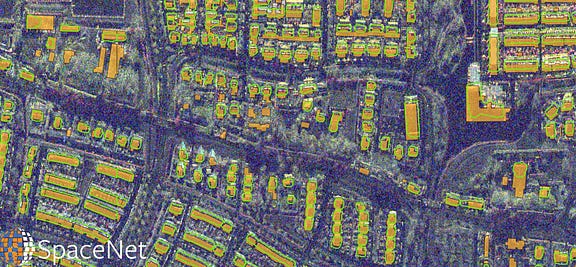
Epilogue

A few more broad scale output images for fun.

Predicting building footprints with SAR at broad scales: All building footprint predictions from the SpaceNet 6 winning algorithm are colorized in red and overlaid upon Maxar WorldView 2 imagery.

Predicting building footprints with SAR for the full testing area: All building footprint predictions from the SpaceNet 6 winning algorithm are colorized in red and overlaid upon Maxar WorldView 2 imagery. Note that some areas are unmapped as they were masked out due to lower fidelity ground-truth.